4 Probability Random Variable A random variable X on a sample space Ω \Omega Ω X : Ω → R X:\Omega\rightarrow R X : Ω → R ω ∈ Ω \omega \in \Omega ω ∈ Ω X ( ω ) X(\omega) X ( ω )
Let a be any number in the range of a random variable X. Then X ( ω ) = a X(\omega) = a X ( ω ) = a
The distribution of a discrete random variable X is the collection of values
{ ( a , P [ X = a ] ) } \{(a,P[X = a])\} {( a , P [ X = a ])} ∈ \in ∈
probability mass function(p.m.f ) P [ X = a ] = p ( a ) P[X=a] = p(a) P [ X = a ] = p ( a )
Expectations and Variance E ( X ) = ∑ x ∈ X ( Ω ) x p ( x ) V a r ( X ) = E [ ( X − E ( X ) ) 2 ] = E ( X 2 ) − E 2 ( X ) E(X) =\sum_{x\in X(\Omega)} xp(x) \\ Var(X) = E[(X - E(X))^2] = E(X^2) - E^2(X) E ( X ) = x ∈ X ( Ω ) ∑ x p ( x ) Va r ( X ) = E [( X − E ( X ) ) 2 ] = E ( X 2 ) − E 2 ( X ) Distribution X ∼ Bernoulli(p) one if a coin with heads probability p comes up heads, zero otherwise.
P [ X = i ] = { p , i = 1 1 − p , i = 0 E ( X ) = p V a r ( X ) = p ( 1 − p ) \begin{aligned} P[X=i]= \begin{cases} p, & i=1 \\ 1-p, & i=0 \end{cases} \\ E(X)=p \\ Var(X)=p(1-p) \end{aligned} P [ X = i ] = { p , 1 − p , i = 1 i = 0 E ( X ) = p Va r ( X ) = p ( 1 − p ) X ∼ Binomial(n, p) n times Bernoulli experiments
P [ X = i ] = ( n i ) p i ( 1 − p ) n − i i =0,1,...,n E ( X ) = n p V a r ( X ) = n p ( 1 − p ) \begin{aligned} P[X=i] =( \begin{matrix} n\\i \end{matrix} )p^i(1-p)^{n-i} \qquad \text{i =0,1,...,n}\\ E(X) = np \\ Var(X) = np(1-p) \end{aligned} P [ X = i ] = ( n i ) p i ( 1 − p ) n − i i =0,1,...,n E ( X ) = n p Va r ( X ) = n p ( 1 − p ) X ∼ Geometric(p) For λ > 0 \lambda > 0 λ > 0
P [ X = i ] = ( 1 − p ) i − 1 p i = 1,2,3,.. E ( X ) = 1 p V a r ( X ) = 1 − p p 2 \begin{aligned} P[X = i]= (1− p)^{i-1}p \qquad \text{i = 1,2,3,..} \\ E(X) = \frac{1}{p} \\ Var(X) = \frac{1-p}{p^2} \end{aligned} P [ X = i ] = ( 1 − p ) i − 1 p i = 1,2,3,.. E ( X ) = p 1 Va r ( X ) = p 2 1 − p X ∼ Poisson(λ \lambda λ P [ X = i ] = λ i i ! e − λ i=0,1,2,... E ( X ) = V a r ( X ) = λ \begin{aligned} P[X = i]= \frac{\lambda^i}{i!}e^{-\lambda} \qquad \text{i=0,1,2,...} \\ E(X) = Var(X) = \lambda \end{aligned} P [ X = i ] = i ! λ i e − λ i=0,1,2,... E ( X ) = Va r ( X ) = λ Continuous Variable A probability density function(PDF ) for a real-valued random variable X is a function f : R → R f:R\rightarrow R f : R → R
f X ( x ) ≥ 0 f_X(x) \geq 0 f X ( x ) ≥ 0 x ∈ R x \in R x ∈ R ∫ − ∞ ∞ f X ( x ) d x = 1 \int_{-\infty}^{\infty}f_X(x)dx = 1 ∫ − ∞ ∞ f X ( x ) d x = 1 Then the distribution of X is given by P [ a ≤ X ≤ b ] = ∫ a b f X ( x ) d x P[a\leq X\leq b] = \int_a^b f_X(x)dx P [ a ≤ X ≤ b ] = ∫ a b f X ( x ) d x
cumulative distribution function(CDF ) F X ( x ) = P ( X ≤ x ) = ∫ − ∞ x f X ( z ) d z F_X(x) = P(X\leq x) = \int_{-\infty}^xf_X(z)dz F X ( x ) = P ( X ≤ x ) = ∫ − ∞ x f X ( z ) d z
E ( x ) = ∫ − ∞ ∞ x f X ( x ) d x E(x) = \int_{-\infty}^{\infty}xf_X(x)dx E ( x ) = ∫ − ∞ ∞ x f X ( x ) d x
Distribution f ( x ) = { 1 b − a , a ≤ x ≤ b 0 , o t h e r f(x) = \begin{cases} \frac1{b-a}, & a\leq x\leq b \\ 0, & other \end{cases} f ( x ) = { b − a 1 , 0 , a ≤ x ≤ b o t h er X ∼ Exponential(λ) For λ > 0 \lambda > 0 λ > 0
f ( x ) = { λ e − λ x , x ≥ 0 0 , o t h e r f(x) = \begin{cases} \lambda e^{-\lambda x}, & x\geq 0 \\ 0, & other \end{cases} f ( x ) = { λ e − λ x , 0 , x ≥ 0 o t h er X ∼ Normal(μ , σ 2 \mu,\sigma^2 μ , σ 2 Also known as the Gaussian distribution
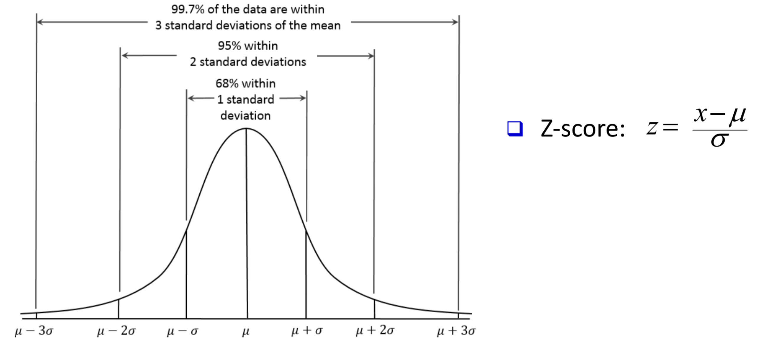
f ( x ) = 1 2 π σ e − ( x − μ ) 2 2 σ 2 f(x) = \frac1{\sqrt{2\pi}\sigma}e^{-\frac{(x-\mu)^2}{2\sigma^2}} f ( x ) = 2 π σ 1 e − 2 σ 2 ( x − μ ) 2
Multiple Variables Joint distribution Random Joint distribution For some random variables X 1 , . . . , X n X_1,...,X_n X 1 , ... , X n p ( X 1 , . . . , X n ) p(X_1,...,X_n) p ( X 1 , ... , X n )
Let { X i } i ∈ I \{X_i\}_{i\in I} { X i } i ∈ I I I I { X i } \{X_i\} { X i } i 1 , . . . , i k ∈ I i_1,..., i_k \in I i 1 , ... , i k ∈ I p ( X i 1 , . . . , X i k ) = ∏ j = 1 k p ( X i j ) p(X_{i1},..., X_{ik}) = \prod_{j=1}^kp(X_{ij}) p ( X i 1 , ... , X ik ) = ∏ j = 1 k p ( X ij )
Marginal distribution p ( X ) = ∑ y p ( X , y ) p(X) = \sum_yp(X,y) p ( X ) = ∑ y p ( X , y )
Continuous Joint distribution For continuous variables, the joint CDF F X Y ( x , y ) = P ( X ≤ x , Y ≤ y ) F_{XY}(x,y) = P(X\leq x, Y\leq y) F X Y ( x , y ) = P ( X ≤ x , Y ≤ y )
the marginal CDF F X ( x ) = lim y → ∞ F X Y ( x , y ) d y F_X(x) = \lim_{y\rightarrow \infty}F_{XY}(x,y)dy F X ( x ) = lim y → ∞ F X Y ( x , y ) d y
In the case that F X Y ( x , y ) F_{XY}(x, y) F X Y ( x , y ) PDF f X Y ( x , y ) = ∂ 2 F X Y ( x , y ) ∂ x ∂ y f_{XY}(x,y) = \frac{\partial^2 F_{XY}(x,y)}{\partial x\partial y} f X Y ( x , y ) = ∂ x ∂ y ∂ 2 F X Y ( x , y )
marginal PDF : f X ( x ) = ∫ − ∞ ∞ f X Y ( x , y ) d y f_X(x) = \int_{-\infty}^{\infty}f_{XY}(x,y)dy f X ( x ) = ∫ − ∞ ∞ f X Y ( x , y ) d y
Conditional Distributions the conditional PDF f Y ∣ X ( y ∣ x ) = f X Y ( x , y ) f X ( x ) f_{Y|X}(y|x) = \frac{f_{XY}(x,y)}{f_X(x)} f Y ∣ X ( y ∣ x ) = f X ( x ) f X Y ( x , y )
Covariance C o v ( X , Y ) = E [ ( X − E ( X ) ) ( Y − E ( Y ) ) ] = E ( X Y ) − E ( X ) E ( Y ) Cov(X,Y) = E[(X-E(X))(Y-E(Y))] = E(XY) - E(X)E(Y) C o v ( X , Y ) = E [( X − E ( X )) ( Y − E ( Y ))] = E ( X Y ) − E ( X ) E ( Y )
correlation ρ ( X , Y ) = C o v ( X , Y ) V a r ( X ) V a r ( Y ) ∈ [ − 1 , 1 ] \rho(X,Y) = \frac{Cov(X,Y)}{\sqrt{Var(X)Var(Y)}} \in [-1,1] ρ ( X , Y ) = Va r ( X ) Va r ( Y ) C o v ( X , Y ) ∈ [ − 1 , 1 ]
s e t Z = ( X − E ( X ) ) t + ( Y − E ( Y ) ) E ( Z 2 ) = V a r ( X ) t 2 + 2 C o v ( X , Y ) t + V a r ( Y ) ≥ 0 ⇒ 4 C o v 2 ( X , Y ) − 4 V a r ( X ) V a r ( Y ) ≤ 0 \begin{aligned} set Z = (X-E(X))t + (Y-E(Y)) \\ E(Z^2) = Var(X)t^2 + 2Cov(X,Y)t + Var(Y) \geq 0 \\ \Rightarrow 4Cov^2(X,Y) - 4Var(X)Var(Y) \leq 0 \end{aligned} se tZ = ( X − E ( X )) t + ( Y − E ( Y )) E ( Z 2 ) = Va r ( X ) t 2 + 2 C o v ( X , Y ) t + Va r ( Y ) ≥ 0 ⇒ 4 C o v 2 ( X , Y ) − 4 Va r ( X ) Va r ( Y ) ≤ 0 We can define Inner product ⟨ X , Y ⟩ : = E ( X Y ) \langle X,Y\rangle:=E(XY) ⟨ X , Y ⟩ := E ( X Y ) c o s θ = ⟨ X − E ( X ) , X − E ( X ) ⟩ ⟨ Y − E ( Y ) , Y − E ( Y ) ⟩ V a r ( X ) V a r ( Y ) cos\theta = \frac{\langle X-E(X),X-E(X)\rangle\langle Y-E(Y),Y-E(Y)\rangle}{Var(X)Var(Y)} cos θ = Va r ( X ) Va r ( Y ) ⟨ X − E ( X ) , X − E ( X )⟩ ⟨ Y − E ( Y ) , Y − E ( Y )⟩
If ρ 2 = 1 \rho^2 = 1 ρ 2 = 1
V a r ( Y − a X ) = V a r ( Y ) + a 2 V a r ( X ) − 2 a C o v ( X , Y ) = V a r ( Y ) + a 2 V a r ( X ) − 2 a ρ V a r ( X ) V a r ( Y ) = ( a V a r ( X ) − ρ V a r ( Y ) ) 2 \begin{aligned} Var(Y-aX) = Var(Y) + a^2Var(X) - 2aCov(X,Y) \\ = Var(Y) + a^2Var(X) - 2a\rho Var(X)Var(Y) \\ = (a\sqrt{Var(X)} - \rho \sqrt{Var(Y)})^2 \end{aligned} Va r ( Y − a X ) = Va r ( Y ) + a 2 Va r ( X ) − 2 a C o v ( X , Y ) = Va r ( Y ) + a 2 Va r ( X ) − 2 a ρ Va r ( X ) Va r ( Y ) = ( a Va r ( X ) − ρ Va r ( Y ) ) 2 if we choose a = ρ V a r ( Y ) V a r ( X ) a = \frac{\rho \sqrt{Var(Y)}}{\sqrt{Var(X)}} a = Va r ( X ) ρ Va r ( Y ) V a r ( Y − a x ) = 0 ⇒ Y = a X Var(Y-ax) = 0 \Rightarrow Y=aX Va r ( Y − a x ) = 0 ⇒ Y = a X
If ρ = 0 \rho = 0 ρ = 0
if X ∼ Uniform(−1, 1) and Y = X 2 Y = X^2 Y = X 2
For multiple variables, define covariance matrix. It is symmetric and semi-definite (for any x, x T Σ x ≥ 0 x^T\Sigma x \geq 0 x T Σ x ≥ 0
Σ = E [ ( X − E ( X ) ) ( X − E ( X ) ) T ] = [ V a r ( X 1 ) C o v ( X 1 , X 2 ) ⋯ C o v ( X 1 , X n ) C o v ( X 2 , X 1 ) V a r ( X 2 ) ⋯ C o v ( X 2 , X n ) ⋮ ⋮ ⋱ ⋮ C o v ( X n , X 1 ) C o v ( X n , X 2 ) ⋯ V a r ( X n ) ] \Sigma = E[(X-E(X))(X-E(X))^T] = \left[ \begin{matrix} Var(X_1) & Cov(X_1, X_2) & \cdots & Cov(X_1, X_n)\\ Cov(X_2, X_1) & Var(X_2) & \cdots & Cov(X_2, X_n)\\ \vdots & \vdots & \ddots & \vdots\\ Cov(X_n, X_1) & Cov(X_n, X_2)& \cdots & Var(X_n) \end{matrix} \right] Σ = E [( X − E ( X )) ( X − E ( X ) ) T ] = ⎣ ⎡ Va r ( X 1 ) C o v ( X 2 , X 1 ) ⋮ C o v ( X n , X 1 ) C o v ( X 1 , X 2 ) Va r ( X 2 ) ⋮ C o v ( X n , X 2 ) ⋯ ⋯ ⋱ ⋯ C o v ( X 1 , X n ) C o v ( X 2 , X n ) ⋮ Va r ( X n ) ⎦ ⎤ Independence Two random variables X and Y are independent if F X Y ( x , y ) = F X ( x ) F Y ( y ) F_{XY}(x, y) = F_X(x)F_Y(y) F X Y ( x , y ) = F X ( x ) F Y ( y )
For discrete random variables, p ( x , y ) = p ( x ) p ( y ) p(x,y) = p(x)p(y) p ( x , y ) = p ( x ) p ( y ) For continuous variables, f X Y ( x , y ) = f X ( x ) f Y ( y ) f_{XY}(x, y) = f_X(x)f_Y(y) f X Y ( x , y ) = f X ( x ) f Y ( y ) The Gaussian distribution p ( x ; μ , Σ ) = 1 ( 2 π ) d det Σ exp ( − 1 2 ( x − μ ) T Σ − 1 ( x − μ ) ) p(x; \mu, \Sigma) = \frac1{\sqrt{(2\pi)^d \det{\Sigma}}}{\exp(-\frac12(x-\mu)^T\Sigma^{-1}(x-\mu))} p ( x ; μ , Σ ) = ( 2 π ) d d e t Σ 1 exp ( − 2 1 ( x − μ ) T Σ − 1 ( x − μ ))
Estimation of Parameters Maximum Likelihood estimation We make some assumptions about our problem by prescribing a parametric model, then we fit the parameters of the model to the data. How do we choose the values of the parameters?
A common way to fit parameters is maximum likelihood estimation (MLE).
Suppose we have random variables X 1 , . . . , X n X_1, . . . , X_n X 1 , ... , X n x 1 , . . . , x n x_1, . . . , x_n x 1 , ... , x n
L ( θ ) = p ( x 1 , . . . , x n ; θ ) L(\theta) = p(x_1, . . . , x_n;\theta) L ( θ ) = p ( x 1 , ... , x n ; θ )
We assume X 1 , . . . , X n X_1, . . . , X_n X 1 , ... , X n
L ( θ ) = ∏ i = 1 n p ( x i ; θ ) log L ( θ ) = ∑ i = 1 n log p ( x i ; θ ) θ m l e = arg max L ( θ ) \begin{aligned} L(\theta) = \prod_{i=1}^np(x_i;\theta)\\ \log L(\theta) = \sum_{i=1}^n\log p(x_i;\theta) \\ \theta _{mle} = \arg\max L(\theta) \end{aligned} L ( θ ) = i = 1 ∏ n p ( x i ; θ ) log L ( θ ) = i = 1 ∑ n log p ( x i ; θ ) θ m l e = arg max L ( θ ) Entropy Information: How uncertain we are of the outcome of random experiments
Self information: i ( x ) = − log 2 p ( x ) i(x) = - \log_2p(x) i ( x ) = − log 2 p ( x )
Entropy
H ( X ) = E [ i ( x ) ] = − ∑ x ∈ X ( Ω ) p ( x ) log 2 p ( x ) H ( X , Y ) = − ∑ y ∈ y ( Ω ) ∑ x ∈ X ( Ω ) p ( x , y ) log 2 p ( x , y ) H ( X ∣ Y ) = − ∑ y ∈ y ( Ω ) ∑ x ∈ X ( Ω ) p ( x , y ) log 2 p ( x ∣ y ) H ( X , Y ) = H ( X ) + H ( Y ∣ X ) = H ( Y ) + H ( X ∣ Y ) \begin{aligned} H(X) = E[i(x)] = -\sum_{x\in X(\Omega)}p(x)\log_2p(x) \\ H(X,Y) = -\sum_{y\in y(\Omega)}\sum_{x\in X(\Omega)}p(x,y)\log_2p(x,y) \\ H(X|Y) = -\sum_{y\in y(\Omega)}\sum_{x\in X(\Omega)}p(x,y)\log_2p(x|y) \\ H(X,Y) = H(X) + H(Y|X) = H(Y) + H(X|Y) \end{aligned} H ( X ) = E [ i ( x )] = − x ∈ X ( Ω ) ∑ p ( x ) log 2 p ( x ) H ( X , Y ) = − y ∈ y ( Ω ) ∑ x ∈ X ( Ω ) ∑ p ( x , y ) log 2 p ( x , y ) H ( X ∣ Y ) = − y ∈ y ( Ω ) ∑ x ∈ X ( Ω ) ∑ p ( x , y ) log 2 p ( x ∣ y ) H ( X , Y ) = H ( X ) + H ( Y ∣ X ) = H ( Y ) + H ( X ∣ Y ) Relative Entropy Jensen's inequality: Let X be a random variable and f(x) be a convex function, then
E ( f ( X ) ) ≥ f ( E ( X ) ) E(f(X))\geq f(E(X)) E ( f ( X )) ≥ f ( E ( X )) Conversely, if f(x) is a concave function
E ( f ( X ) ) ≤ f ( E ( X ) ) E(f(X))\leq f(E(X)) E ( f ( X )) ≤ f ( E ( X )) Relative Entropy (Kullback-Leibler divergence):
D ( p ( x ) ∣ ∣ q ( x ) ) = ∑ x ∈ X ( Ω ) p ( x ) log p ( x ) q ( x ) = − E p [ log q ( x ) p ( x ) ] ≥ − log E p [ q ( x ) p ( x ) ] ≥ 0 D(p(x)||q(x)) = \sum_{x\in X(\Omega)}p(x)\log\frac{p(x)}{q(x)} = - E_p[\log\frac{q(x)}{p(x)}] \geq -\log E_p[\frac{q(x)}{p(x)}] \geq 0 D ( p ( x ) ∣∣ q ( x )) = x ∈ X ( Ω ) ∑ p ( x ) log q ( x ) p ( x ) = − E p [ log p ( x ) q ( x ) ] ≥ − log E p [ p ( x ) q ( x ) ] ≥ 0 Connection to MLE Set loss function loss( x ) = − log q ( x ) (x) = -\log q(x) ( x ) = − log q ( x )
Risk( q ) = − E p ( log q ( x ) ) = D ( p ∣ ∣ q ) + (q) = -E_p(\log q(x))= D(p||q) + ( q ) = − E p ( log q ( x )) = D ( p ∣∣ q ) + ( p ) (p) ( p )
Thus, arg min D ( p ∣ ∣ q ) = arg min \arg \min D(p||q) = \arg \min arg min D ( p ∣∣ q ) = arg min ( q ) (q) ( q )
Here, we call Risk(q) as cross entropy CE(p,q)