2 Graph
Graph
Definition
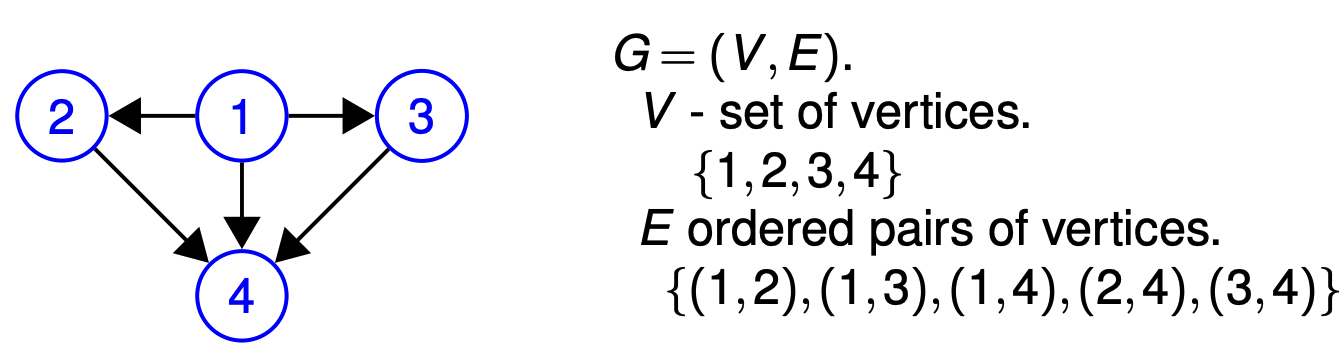
Graph: 𝐺 = (𝑉, 𝐸)
- V: set of vertices.
- (set of edges)
if and , we call e as "loop"
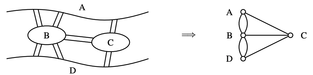
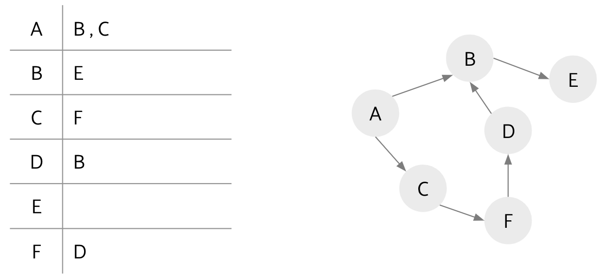
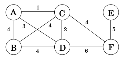
In Figure 1, V = {A,B,C,D} and E = {{A,B},{A,B},{A,C},{B,C},{B,D},{B,D},{C,D}}.
Here, E is a multiset.
If there are no loops and E is a set(no parallel edges), then G is a simple graph.
- u is neighbor of v if , edge is incident to u and v.
- Degree of vertex u is number of incident edges
In directed graph, each defined as .
- the in-degree of a vertex u is the number of edges from other vertices to u, and the out-degree of u is the number of edges from u to other vertices.
Paths, walks, cycles, tour
- Path: a sequence of edges
- Cycle: Path from to , + edge
- Walk is sequence of edges with possible repeated vertex or edge
- Tour is walk that starts and ends at the same node.
Hamiltonian cycle: A cycle that visits every vertex in graph exactly once
Connectivity
u and v are connected if there is a path between u and v
- Connected graph: A graph where all pairs of vertices are connected
- Connected component: Maximal set of connected vertices
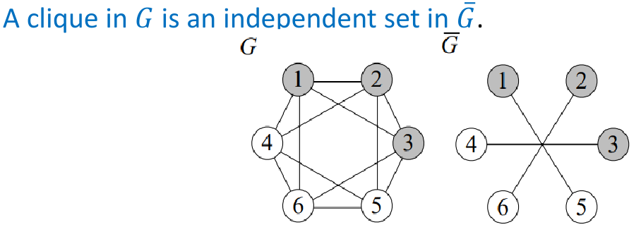
- Independent set: No two vertices are connected by an edge
- Clique: Every pair of vertices is connected by an edge
- Minimum Vertex Cover: for every edge , either or . The task is to find the minimum
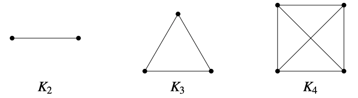
Complete Graph
complete graph on n vertices
every pair of (distinct) vertices u and v are connected by an edge .
Representation
Adjacency matrices are true if there is a line going from node A to B and false otherwise
Adjacency lists list out all the nodes connected to each node in our graph
Searching
DFS and BFS runtime with adjacency list: O(V + E) (creating marked array)
DFS and BFS runtime with adjacency matrix: O()
DFS is worse for spindly graphs (Θ(V) memory to remember recursive calls)
BFS is worse for absurdly “bushy” graphs (In worst case, queue will require Θ(V) memory.)
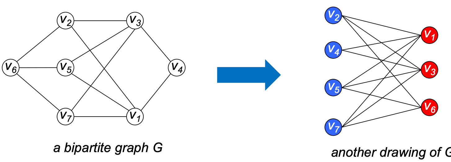
Bipartite
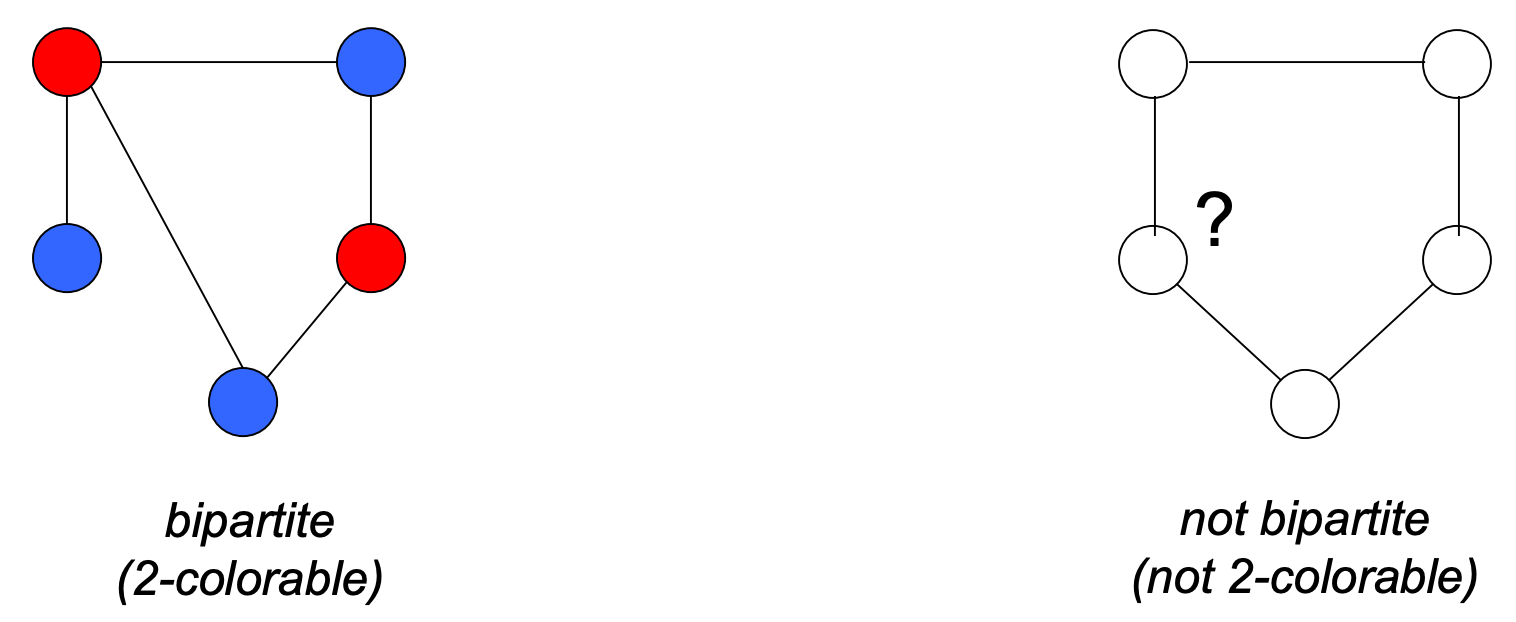
An undirected graph 𝐺 = (𝑉, 𝐸) is bipartite if you can partition the vertex set into 2 parts so that all edges join vertices in different parts
A graph G is bipartite if and only if it contains no odd length cycles.
Proof:
(1) If G is bipartite, then it does not contain an odd length cycle.
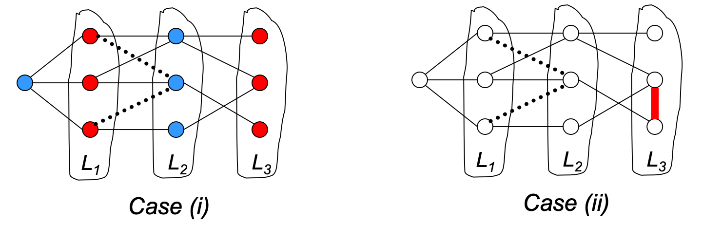
(2) Let G be a connected graph, and let be the layers produced by BFS.
Then only 2 situations:
- No edge of G joins two nodes of the same layer, and G is bipartite. See blue and red parts.
- An edge of G joins two nodes of the same layer, and G contains an odd-length cycle (and hence is not bipartite). Consider the edge and the lowest common ancestor of the connecting vertices. The total length must be odd.
BFS solution to test bipartiteness:
队首孩子结点入队时, 判断是否在同一层
Shortest Path
Dijkstra's algorithm /ˈdaɪkstrə/
int dijkstra(){
    PQ.push({source, 0});
    while(!PQ.empty()){
        p = PQ.top();
        PQ.pop();
        for (q:adjlist[p]){
            if (distTo[p] + w < distTo[q]){
                distTo[q] = distTo[p] + w; // relax
                edgeTo[q] = p;
                PQ.push({q, distTo[q]});
            }
        }
    }
}
Dijkstra’s is guaranteed to return a correct result if all edges are non-negative
Proof:
After relaxing all edges from source, let vertex v1 be the vertex with minimum weight(closest to the source)
Claim: distTo[v1] is optimal, and thus future relaxations will fail
- distTo[p] ≥ distTo[v1] for all p, therefore
- distTo[p] + w ≥ distTo[v1]
Runtime:
- removeSmallest: V times, each costing O(log V) time.
- changePriority: E times, each costing O(log V) time.
Assuming E > V, this is just O(Elog V) for a connected graph
DAG
Directed acyclic graph
Topological sort: order the vertices one after the other in such a way that each edge goes from an earlier vertex to a later vertex
A topological sort only exists if the graph is a DAG
Property: Every dag has at least one source and at least one sink(proof easy)
- O(V+E) time
- Θ(V) space
Solution
- BFS
- DFS
- process all of the edges and keep a count of the number of incoming edges for each node
- Find a source, output it, and delete it from the graph
- The graph is still a DAG, and thus will still have a source vertex
- Repeat until the graph is empty
bool topolical_sort(){
    // graph可包含self cycle and parallel edge
    queue<int> q;
    // find source
    for (int i = 0; i < indegree.size(); ++i) {
        if (!indegree[i]) q.push(i);
    }
    // repeating pop source
    while (!q.empty()) {
        int u = q.front();
        res.push_back(u);
        q.pop();
        for (auto v: graph[u]){
            --indegree[v];
            if (!indegree[v]) q.push(v);
        }
    }
    // Check DAG
    return res.size()==n;
}
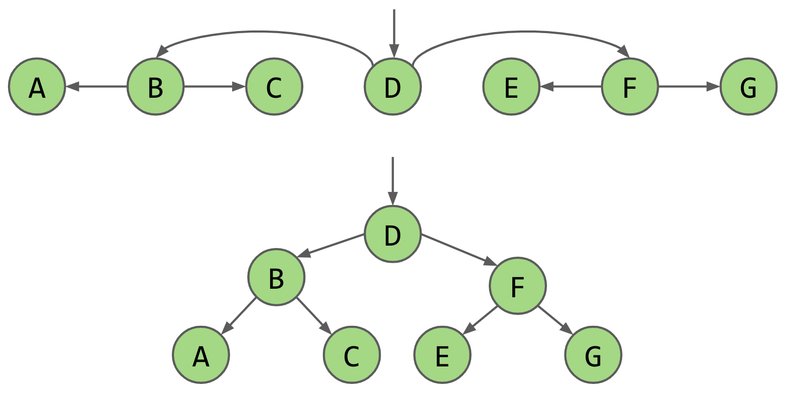
- Perform a DFS traversal from an arbitrary vertex, record DFS postorder in a list
- If not all marked, pick an unmarked vertex and do it again
- Topologica lordering is given by the reverse of that list
Shortest path on DAG
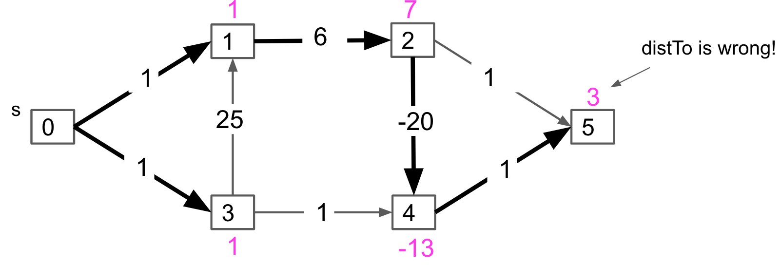
Dijkstra may suffer from negative edges(dist to 5 is update earlier than 2)
Solution: visit all the vertices in topological order, relaxing all edges as we go
- O(V+E) time
- Θ(V) space
Longest path on DAG: just flip all weights and treat as SPT
Tree
A connected graph without a cycle
or: A connected graph with |V| −1 edges.
Binary Tree
Tree Terminology
- The depth of a node is the number of edges from the root to the node
- The height of a node is the number of edges from the node to the deepest leaf
- The height of a tree is a height of the root
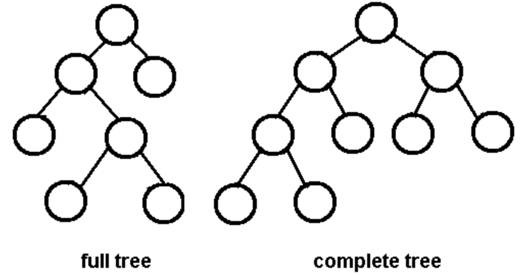
- A full binary tree is a binary tree in which each node has exactly zero or two children
- A complete binary tree is a binary tree, which is completely filled, with the possible exception of the bottom level, which is filled from left to right
Tree traversals
A traversal is a process that visits all the nodes in the tree
- depth-first traversal
- PreOrder traversal
- InOrder traversal
- PostOrder traversal
- breadth-first traversal
- For binary tree, BFS = level order traversal
BST
Binary search in ordered linked list
Move pointer to middle and flip left links
Binary Search Tree
A BST is a binary tree where nodes are ordered in the following way:
- Every key in the left subtree is less than X's key
- Every key in the right subtree is greater than X's key
insert
insert(BST T, Key ik) {
    if (T == null)
        return new BST(ik);
    if (ik ≺ T.key)
        T.left = insert(T.left, ik);
    else if (ik ≻ T.key)
        T.right = insert(T.right, ik);
    return T;
}
delete
Deletion with two Children(Hibbard)
If we want to delete k, move g or m upward
Implement Map
To represent maps, just have each BST node store key/value pairs
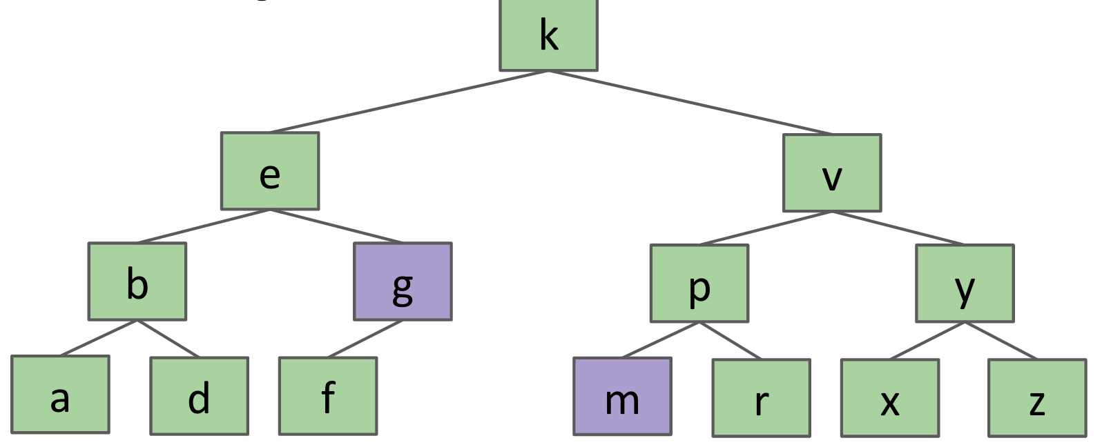
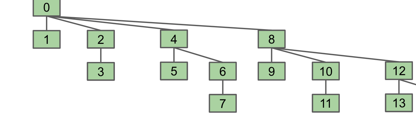
Tree Height
- Θ(log N) in the best case (Left: "bushy")
- Θ(N) in the worst case (Right: "spindly")
- Θ(log N) height if constructed via random inserts
BST Rotation
rotateLeft(G): Head->Left Child
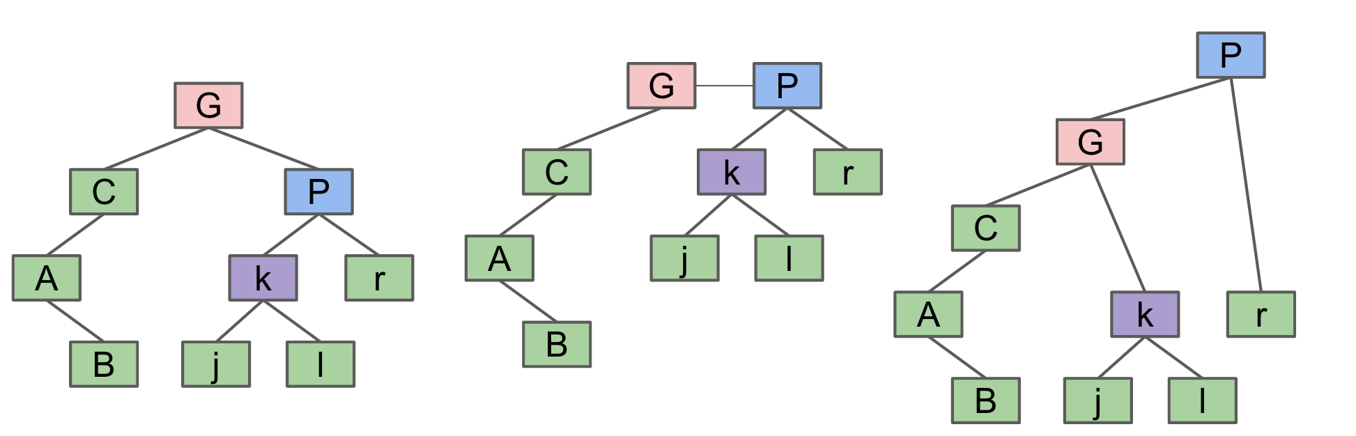
rotateRight(P): Head->Right Child
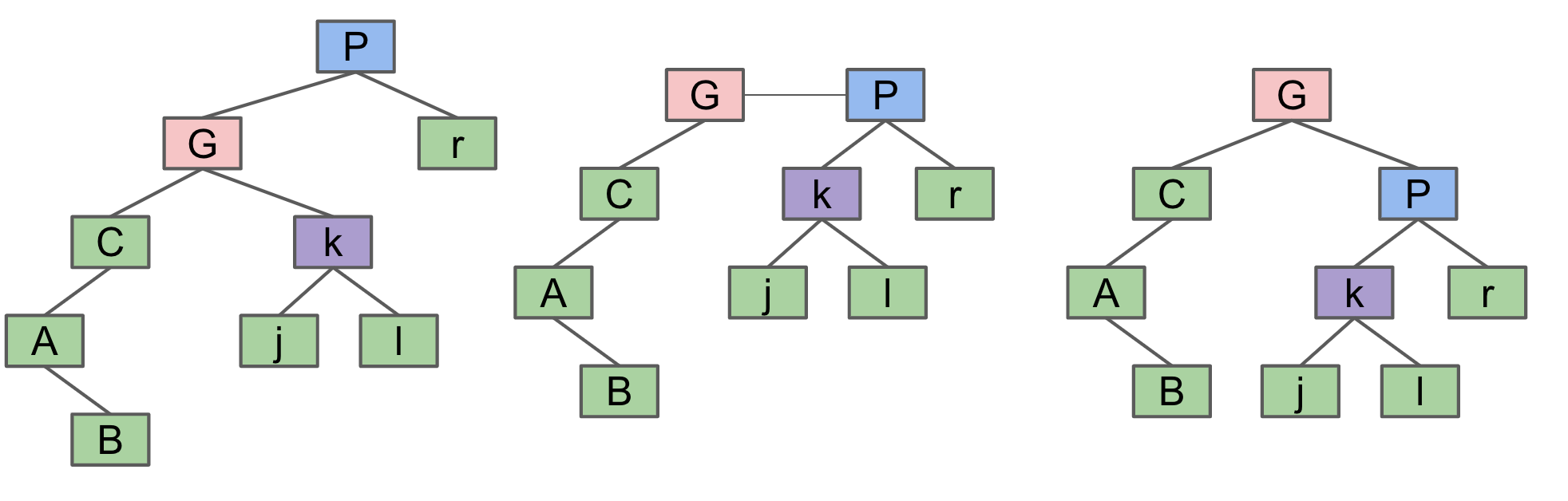
Rotation:
- Can shorten (or lengthen) a tree
- Preserves search tree property
BTree
Concept
Problem with BST: Adding new leaves at the bottom makes it imbalanced -> Avoid new leaves by "overstuffing" the leaf nodes
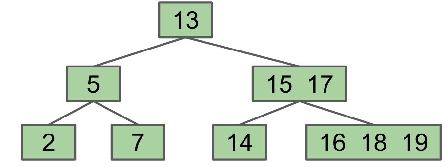
Height is balanced, but leaf nodes can get too juicy
Solution: Set a limit L on the number of items, say L=3, move the left-middle
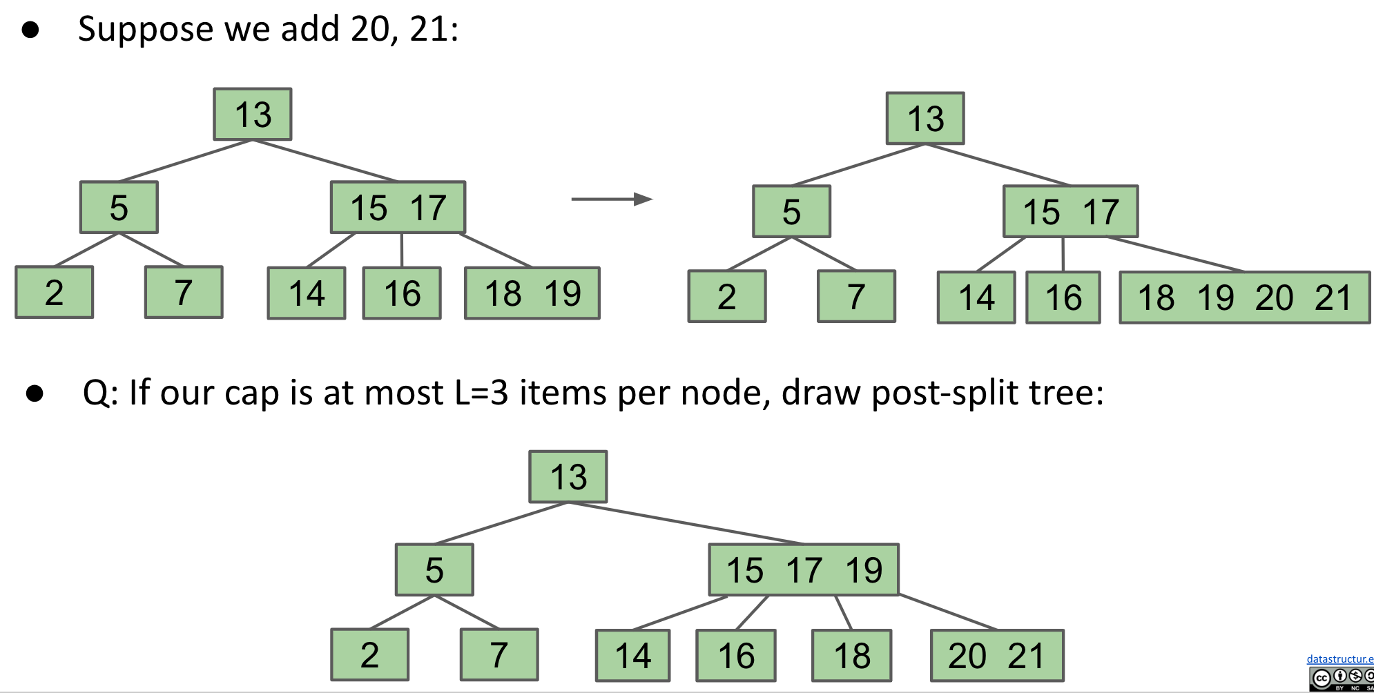
B(balanced/bushy)-trees of order L=3 are also called a 2-3-4(number of children) tree or a 2-4 tree
B-Tree Runtime Analysis
The minimum degree of the B-tree t is an integer such that:
- Every node other than the root must have at least t - 1 keys
- Every internal node other than the root must have at least t children
- The root must have at least one key
Height:
H = O(log n)
Contains:
- Worst case number of nodes to inspect: H + 1
- Worst case number of items to inspect per node: L
- Overall runtime: O(HL) = O(log n)
Add:
- Worst case number of nodes to inspect: H + 1
- Worst case number of items to inspect per node: L
- Worst case number of split operations: H + 1
- Overall runtime: O(HL) = O(log n)
Red-Black Trees
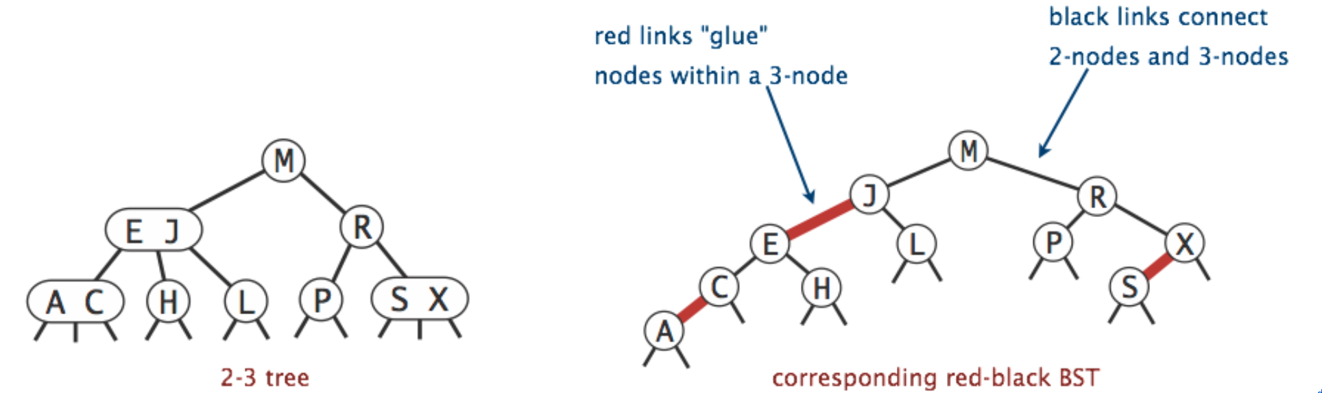
Representing a 2-3 Tree as a BST
- Binary search trees: Can balance using rotation
- 2-3 Tree: Balanced by construction
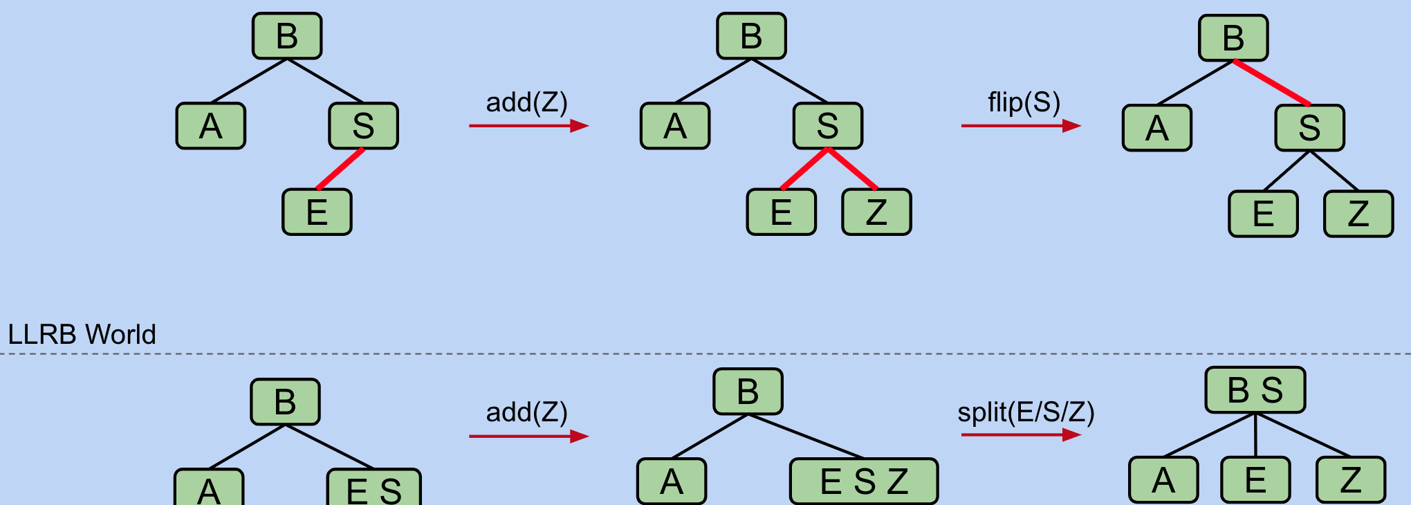
Solution: Create "glue"(red) links with the smaller item off to the left
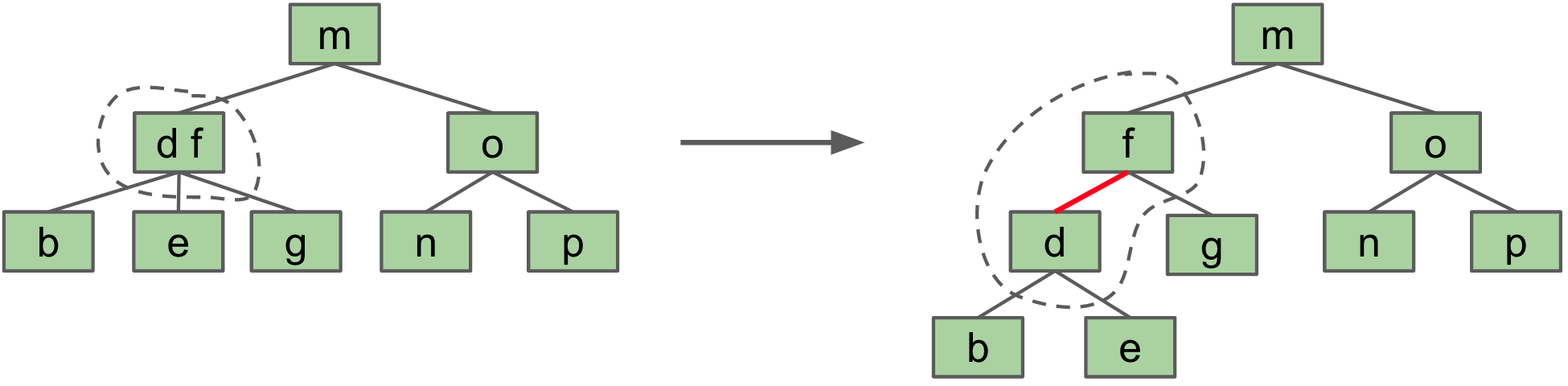
Left-Leaning Red Black Binary Search Tree (LLRB)
There is a 1-1 correspondence between an LLRB and an equivalent 2-3 tree
private class Node {
    private Key key;           // key
    private Value val;         // associated data
    private Node left, right;  // links to left and right subtrees
    private boolean color;     // color of parent link
    private int size;          // subtree count

    public Node(Key key, Value val, boolean color, int size) {
        this.key = key;
        this.val = val;
        this.color = color;
        this.size = size;
    }
}
LLRB Height
LLRB has no more than ~2x the height of its 2-3 tree: O(log n)
Insertion
Use red link
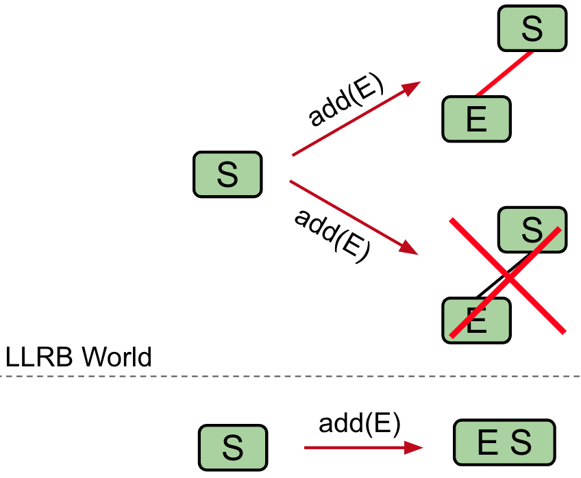
Insertion on the Right
If there is a right leaning "3-node", Rotate left the appropriate node to fix
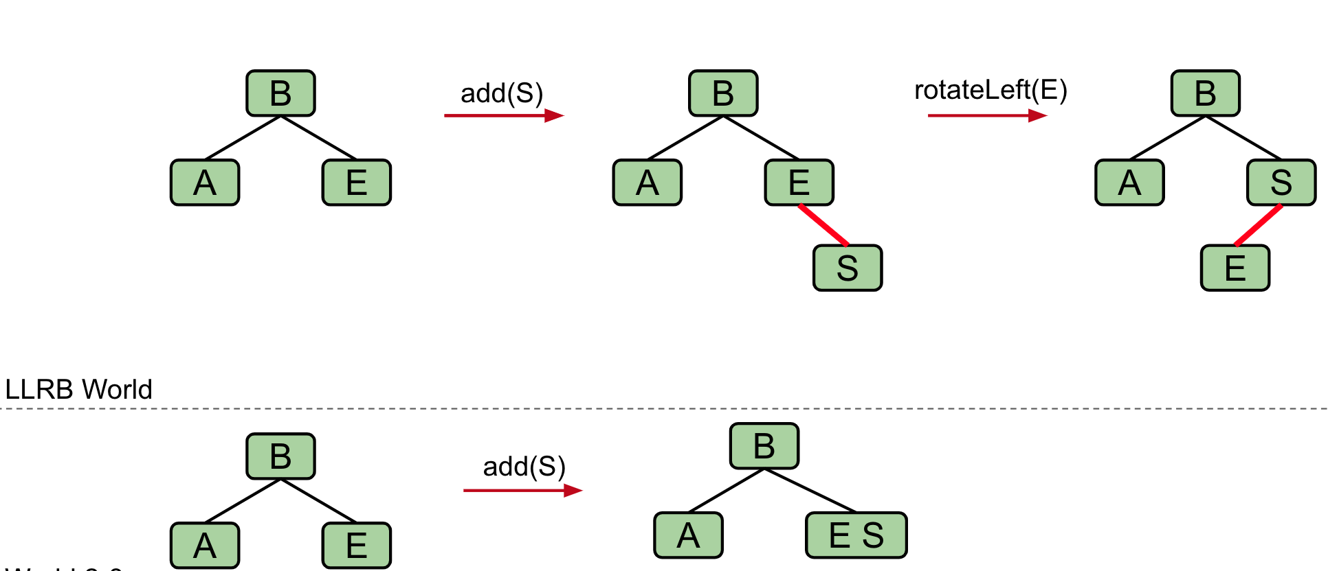
private Node rotateLeft(Node h) {
    assert (h != null) && isRed(h.right);
    Node x = h.right;
    h.right = x.left;
    x.left = h;
    x.color = h.color;
    h.color = RED;
    x.size = h.size;
    h.size = size(h.left) + size(h.right) + 1;
    return x;
}
Double Insertion on the Left
If there are two consecutive left links, rotate right the appropriate node to fix
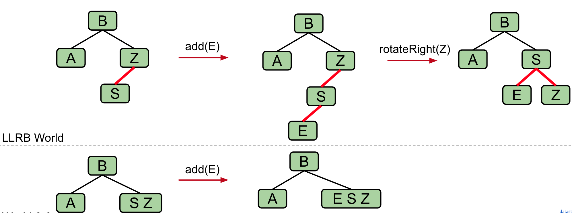
private Node rotateRight(Node h) {
    assert (h != null) && isRed(h.left);
    Node x = h.left;
    h.left = x.right;
    x.right = h;
    x.color = h.color;
    h.color = RED;
    x.size = h.size;
    h.size = size(h.left) + size(h.right) + 1;
    return x;
}
Splitting 4-Nodes
If there are any nodes with two red children, color flip
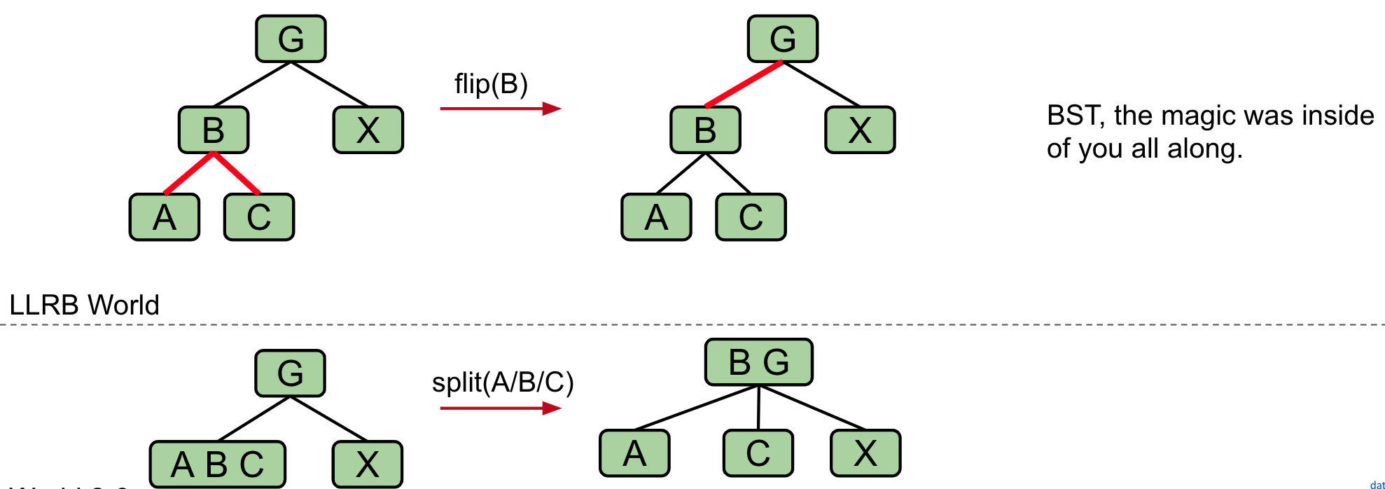
private void flipColors(Node h) {
    h.color = !h.color;
    h.left.color = !h.left.color;
    h.right.color = !h.right.color;
}
Cascading operations
It is possible that a rotation or flip operation will cause an additional violation that needs fixing
Wrapping it up
private Node put(Node h, Key key, Value val) {
    if (h == null) return new Node(key, val, RED, 1);

    int cmp = key.compareTo(h.key);
    if      (cmp < 0) h.left  = put(h.left,  key, val);
    else if (cmp > 0) h.right = put(h.right, key, val);
    else              h.val   = val;

    // fix-up any right-leaning links
    if (isRed(h.right) && !isRed(h.left))      h = rotateLeft(h);
    if (isRed(h.left)  &&  isRed(h.left.left)) h = rotateRight(h);
    if (isRed(h.left)  &&  isRed(h.right))     flipColors(h);
    h.size = size(h.left) + size(h.right) + 1;

    Balance(); // Cascading operations
    return h;
}
LLRB Runtime
- Contains: O(log n)
- Insert:
- O(log n) to add the new node
- O(log n) rotation and color flip operations per insert
Disjoint Sets
int findf(int v){
    if(v!=father[v])
        father[v]=findf(father[v]);//注意点
    return father[v];
}
void uni(int a,int b){
    int fa = findf(a);
    int fb = findf(b);
    if(fa!=fb)
        father[fa] = fb;
}
Improvement: Weighted Quick Union
Modify uni():
- Track tree size (number of elements)
- Always link root of smaller tree to larger tree
Worst case tree height is O(log n)
findf and uni are O(log n)
Minimum Spanning Trees
Input: An undirected graph G = (V, E), edge weights
Output: A tree , with , that minimizes weight
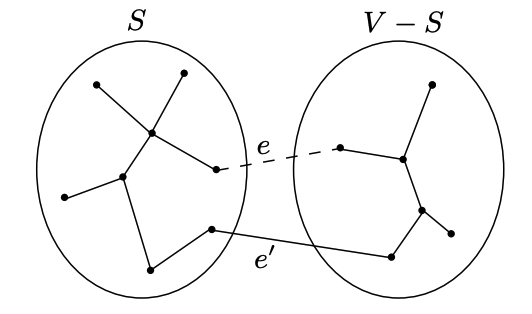
Cut property
A cut is any partition of V into two groups, S and V −S
A crossing edge is an edge which connects a node from S to a node from the V-S
Claim: Given any cut, minimum weight crossing edge is in the MST
Proof:
Suppose a minimum spanning tree doesn't contain e, then there must be some other edge across the cut (S, V −S)
if we remove and add , , then T' must be connected.
And it has the same number of edges as T; so it is also a tree.
but weight weight
Prim's Algorithm
Prim Runtime just as Dijkstra: O(ElogV)
int prism(){
    distTo[s] = 0;
    PQ.push({s,0})

    /* Get vertices in order of distance from tree. */
    while (!PQ.empty()) {
        int v = PQ.top();
        PQ.pop();
        visit[v] = true;
        for (Edge e:adjlist[v]){
            int q = e.head;
            if (!visit[q] && e.weight < distTo[q]) {
                distTo[q] = e.weight;
                edgeTo[q] = e;
                PQ.push({q, distTo[q]});
            }
        }
    }
}
Kruskal's Algorithm
int kruskal(){
    sort(EdgeList.begin(),EdgeList().end());
    for(e:EdgeList){
        int fa = findf(e.from);
        int fb = findf(e.to);
        if(fa!=fb){
            father[e.from] = e.to;
            edgeTo[e.to] = e;
        }
    }
}
Runtime:
- sort: O(ElogE)
- union: O(ElogV)
Assuming E > V, this is just O(ElogE)
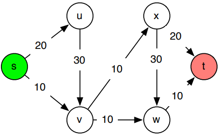
Network Flow
Definition
A flow network is a connected, directed graph G = (V, E).
- Each edge has a capacity
- A single source and a single sink
- No edge enters the source and no edge leaves the sink
Def. A flow is a function that assigns a real number to each edge, satisfying the following two properties
- Capacity: for each edge e
- Conservation: for each vertex except s,t
capacity of the cut: cap(A,B) =
Our task is to maximize the value of the flow
Flow and Cut Lemma
Flow Lemma: Let f be any flow, and let (A, B) be any s-t cut. Then
(Proof Easy)
Cut capacity Lemma: Let f be any flow, and let (A, B) be any s-t cut. Then the value of the flow is at most the capacity of the cut.
cap(A,B)
Residual graph
Residual graph
For an origin edge e = (u, v) in G
- Remaining capacity left: if , copy the edge e with capacity
- Erase origin: if , include an edge e' = (v, u) with capacity
Augmenting Path:
- Let P be an s − t path in the residual graph
- Let bottleneck (P, f) be the smallest capacity in on any edge of P
- We can increase the flow by (P, f)
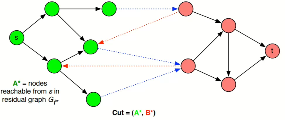
Theorem: maximum flow = minimum cut
Proof: if is maximized, then has no augmenting path
Let denote the set of vertices that are reachable from s: If there is an augmenting path from s to a vertex v then . Also
- Blue edges must be saturated otherwise there would be a forward edge which make an augmenting path
- Red edges must be empty otherwise there would be a forward edge which make an augmenting path
Algorithms
Ford-Fulkerson Algorithm
Runtime: O((E+V)f)
Assuming E > V, this is O(Ef)
int dfs(int s, int t, int flow){
    visit[s] = true;
    for (Edge e:adjlist[s]){
        if(e.weight > 0 && !visit[e.from]){
            int newFlow = dfs(e.to, t, min(flow, e.weight));
            if(newFlow > 0){
                e.weight -= newFlow;
                edge[e.to].weight += newFlow;
                return newFlow;
            }
        }
    }
    return -1;
}
int ff(int s, int t){
    int ans = 0;
    while (1)
    {
        memset(visit, false, sizeof(visit));
        int d = dfs(s, t, inf);
        if (d == -1)
            return ans;
        ans += d;
    }
}