1 Regression and Classification Classification vs Regression:
The target variables in classification are discrete, while in regression are continuous Classes have their order, while Clusters are exchangeable Notations and general concepts L-norm Minkowski distance(L-norm)
def minkowski_distance ( a , b , p ) : return sum ( abs ( e1 - e2 ) ** p for e1 , e2 in zip ( a , b ) ) ** ( 1 / p ) p = 1, Manhattan Distance p = 2, Euclidean Distance Normalization Z score(See probability) Min - max Batch Normalization Internal Covariate Shift(ICS)
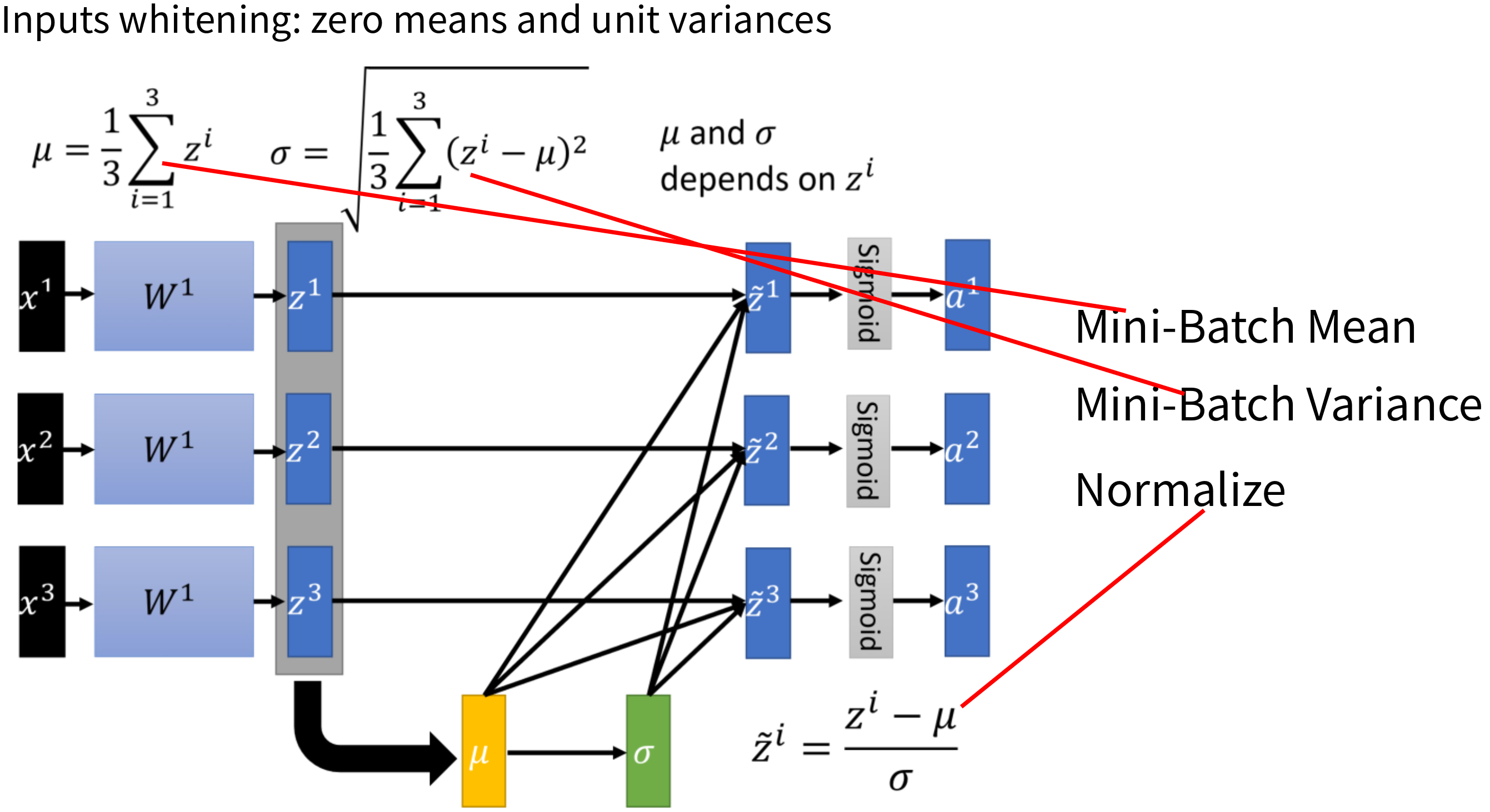
While training a model, we expect independent and identically distributed data For a deep learning model, as the parameter of a lower layer changes, the input distribution of the upper layer also changes. It's called Internal Covariate Shift The upper layer's parameters need to continuously adapt to the new input data distribution, thus reduces the learning speed Problems caused by ICS
Require Lower learning rates: Training would be slower More careful about initializing: saturated regime will slow down the convergence Batch normalization
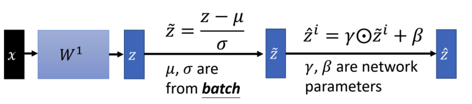
Batch normalize: Calculate mini-batch mean and variance of each layer to decrease covariate shift Scale and shift: Identity transform in order to avoid linear regime of the nonlinearity
Layer Normalization Compute the layer normalization all the hidden units in the same layer
Cross Validation simple cross validation:
Randomly divide training data into S t r a i n S_{train} S t r ain S c v S_{cv} S c v For each model, traing on S t r a i n S_{train} S t r ain Estimate error on validation set S c v S_{cv} S c v find the smallest error K fold cross validation:
Randomly divide training data into k equal parts S 1 , S 2 , . . . , S k S_1,S_2,...,S_k S 1 , S 2 , ... , S k For each model, traing on all the data except S j S_j S j Estimate error on validation set S j S_j S j e r r o r S j error_{S_j} erro r S j Repeat k times, find the smallest error E r r o r = 1 k ∑ i = 1 k e r r o r S j Error = \frac1k \sum_{i=1}^k error_{S_j} E rror = k 1 ∑ i = 1 k erro r S j
Leave-one-out cross validation:
repeatedly train on all but one of the training examples and test on that
held-out example
K fold vs LOO:
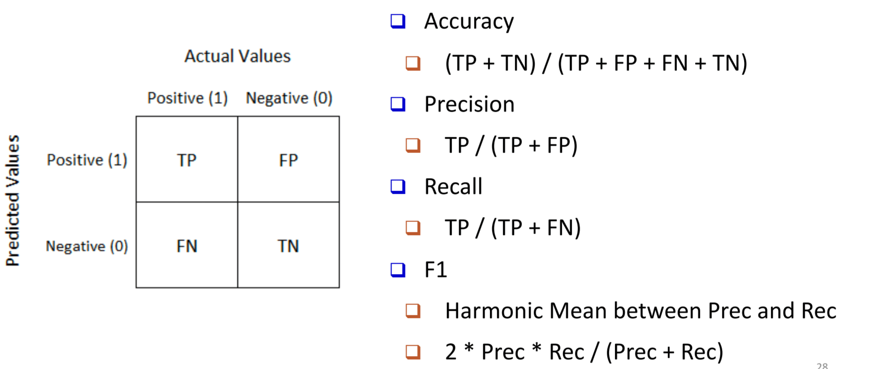
much faster more biased(LOO used in sparse dataset) Metrics Precision: the proportion of correctly predicted positive instances out of all instances the model predicted as positive. Precision i = TP i TP i + FP i \text{Precision}_i = \frac{\text{TP}_i}{\text{TP}_i + \text{FP}_i} Precision i = TP i + FP i TP i Recall: the proportion of correctly predicted positive instances out of all actual positive instances. Recall i = TP i TP i + FN i \text{Recall}_i = \frac{\text{TP}_i}{\text{TP}_i + \text{FN}_i} Recall i = TP i + FN i TP i Macro F1 = 1 n ∑ i = 1 n F1 i \text{Macro F1} = \frac{1}{n} \sum_{i=1}^{n} \text{F1}_i Macro F1 = n 1 ∑ i = 1 n F1 i Macro Precision = 1 n ∑ i = 1 n Precision i \text{Macro Precision} = \frac{1}{n} \sum_{i=1}^{n} \text{Precision}_i Macro Precision = n 1 ∑ i = 1 n Precision i Micro Precision = ∑ c T P c ∑ c T P c + ∑ c F P c \text{Micro Precision} = \frac{\sum_c TP_c}{\sum_c TP_c + \sum_c FP_c} Micro Precision = ∑ c T P c + ∑ c F P c ∑ c T P c Micro Recall = ∑ c T P c ∑ c T P c + ∑ c F N c \text{Micro Recall} = \frac{\sum_c TP_c}{\sum_c TP_c + \sum_c FN_c} Micro Recall = ∑ c T P c + ∑ c F N c ∑ c T P c
Linear Regression Say we find a function f ( x , θ ) = θ T x f(x,\theta) = \theta^T x f ( x , θ ) = θ T x
minimize a loss function L ( θ ) = ∑ i = 1 N l ( f ( x ( i ) , θ ) , y ( i ) ) L(\theta) = \sum_{i=1}^Nl(f(x^{(i)},\theta),y^{(i)}) L ( θ ) = ∑ i = 1 N l ( f ( x ( i ) , θ ) , y ( i ) )
Ordinary Least Square Regression θ : ω , b \theta: \omega,b θ : ω , b l l l L = 1 2 ∑ i = 1 N ( f ( x ( i ) , θ ) − y ( i ) ) 2 L = \frac12\sum_{i=1}^N(f(x^{(i)},\theta) - y^{(i)})^2 L = 2 1 ∑ i = 1 N ( f ( x ( i ) , θ ) − y ( i ) ) 2 1 2 \frac12 2 1
Gradient descent For square loss,
∇ θ L ( θ t ) = ∂ L ( θ ) ∂ θ j = x j ( y − h θ ( x ) ) \nabla_{\theta} L(\theta_t) = \frac{\partial L(\theta)}{\partial \theta_j} = x_j(y-h_{\theta}(x)) ∇ θ L ( θ t ) = ∂ θ j ∂ L ( θ ) = x j ( y − h θ ( x )) Initialize θ 0 \theta_0 θ 0 Repeat: θ t + 1 = θ t − η ∇ θ L ( θ t ) \theta_{t+1} = \theta_{t} - \eta \nabla_{\theta} L(\theta_t) θ t + 1 = θ t − η ∇ θ L ( θ t ) η \eta η
too small: no much progress too big: Overshoot Adjust Learning rate constant learning rate linear decay: linearly decreases over the training period cosine learning rate: a max learning rate times the cosine value(from 0 to 1) adaptive learning rate Adagrad:
η t = η t + 1 , g t = ∇ θ L ( θ t ) θ t + 1 = θ t − η t σ t g t σ t = ∑ i = 0 t g i 2 t + 1 \begin{aligned} \eta_t = \frac{\eta}{\sqrt{t+1}}, g_t = \nabla_{\theta} L(\theta_t) \\ \theta_{t+1} = \theta_t - \frac{\eta_t}{\sigma^t}g_t \\ \sigma_t = \sqrt{\frac{\sum_{i=0}^{t}g^2_i}{t+1}} \end{aligned} η t = t + 1 η , g t = ∇ θ L ( θ t ) θ t + 1 = θ t − σ t η t g t σ t = t + 1 ∑ i = 0 t g i 2 Stochastic Gradient Descent Gradient descent could be slow: Every update involves the entire training data
Stochastic Gradient Descent (SGD)
Sample a batch of training data to estimate ∇ L ( θ t ) \nabla L(\theta_t) ∇ L ( θ t )
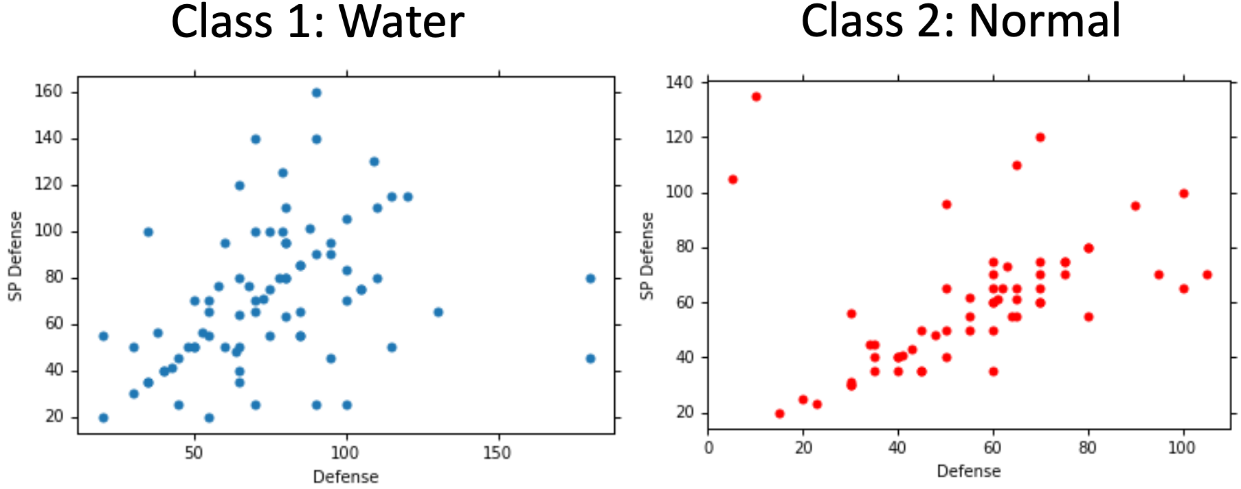
Classification Assume in C1, X ∼ N ( μ 1 , σ 2 ) X \sim N(\mu_1,\sigma^2) X ∼ N ( μ 1 , σ 2 ) X ∼ N ( μ 2 , σ 2 ) X \sim N(\mu_2,\sigma^2) X ∼ N ( μ 2 , σ 2 )
Apply min-max normalization for the target variable → \rightarrow →
Bayes‘ rule:
P ( C 1 ∣ x ) = P ( x ∣ C 1 ) P ( C 1 ) P ( x ∣ C 1 ) P ( C 1 ) + P ( x ∣ C 2 ) P ( C 2 ) P(C_1|x) = \frac{P(x|C_1)P(C_1)}{P(x|C_1)P(C_1) + P(x|C_2)P(C_2)} P ( C 1 ∣ x ) = P ( x ∣ C 1 ) P ( C 1 ) + P ( x ∣ C 2 ) P ( C 2 ) P ( x ∣ C 1 ) P ( C 1 ) we can proof that Logistic Regression
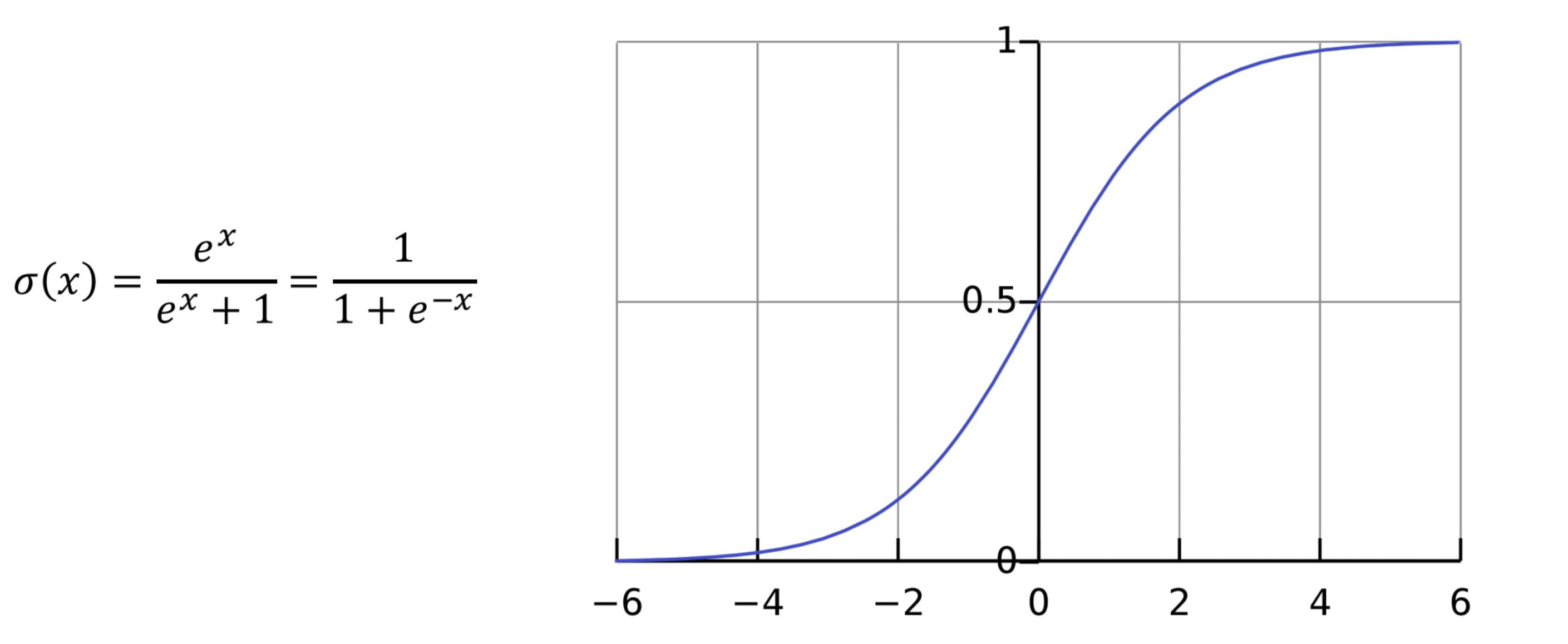
log P ( C 1 ∣ x ) P ( C 2 ∣ x ) = θ T x \log\frac{P(C_1|x)}{P(C_2|x)} = \theta^T x log P ( C 2 ∣ x ) P ( C 1 ∣ x ) = θ T x As
P ( C 1 ∣ x ) + P ( C 2 ∣ x ) = 1 P ( C 1 ∣ x ) = 1 1 + e − θ T x = 1 1 + e − z \begin{aligned} P(C_1|x) + P(C_2|x) = 1 \\ P(C_1|x) = \frac1{1+e^{-{\theta}^Tx}} = \frac1{1+e^{-z}} \end{aligned} P ( C 1 ∣ x ) + P ( C 2 ∣ x ) = 1 P ( C 1 ∣ x ) = 1 + e − θ T x 1 = 1 + e − z 1 We called it "Sigmoid"
Maximum Likelihood Estimate Let us assume that P ( y ∣ x ; θ ) = h θ ( x ) P(y|x;\theta)=h_{\theta}(x) P ( y ∣ x ; θ ) = h θ ( x ) y i = { 0 , 1 } y_i=\{0,1\} y i = { 0 , 1 }
p ( x 1 , x 2 , . . . , x n ; θ ) = ∏ i = 1 n h θ y i ( x i ) ( 1 − h θ ( x i ) ) 1 − y i p(x_1,x_2,...,x_n;\theta) = \prod_{i=1}^n h_{\theta}^{y_i}(x_i)(1-h_{\theta}(x_i))^{1-y_i} p ( x 1 , x 2 , ... , x n ; θ ) = i = 1 ∏ n h θ y i ( x i ) ( 1 − h θ ( x i ) ) 1 − y i Cross-Entropy Loss
L ( θ ) = log p ( x 1 , x 2 , . . . , x n ; θ ) = ∑ i = 1 n y i log h θ ( x i ) + ( 1 − y i ) log ( 1 − h θ ( x i ) ) L(\theta) = \log p(x_1,x_2,...,x_n;\theta) = \sum_{i=1}^n y_i\log h_{\theta}(x_i) + (1-y_i)\log (1-h_{\theta}(x_i)) L ( θ ) = log p ( x 1 , x 2 , ... , x n ; θ ) = i = 1 ∑ n y i log h θ ( x i ) + ( 1 − y i ) log ( 1 − h θ ( x i )) Then
∂ L ( θ ) ∂ θ j = x j ( y − h θ ( x ) ) \frac{\partial L(\theta)}{\partial \theta_j} = x_j(y-h_{\theta}(x)) ∂ θ j ∂ L ( θ ) = x j ( y − h θ ( x )) same as gradient descent
Multiclass Classification If we look at sigmoid function P ( y 1 ∣ x ) = e θ T x e θ T x + 1 P(y_1|x) = \frac{e^{\theta^Tx}}{e^{\theta^Tx} + 1} P ( y 1 ∣ x ) = e θ T x + 1 e θ T x
P ( y ∣ x ; θ ) = exp ( θ T x ⃗ ) ∑ j = 1 n exp ( θ j T x ) P(y|x;\theta) = \frac{\exp(\vec{\theta^T x})}{\sum_{j=1}^n\exp(\theta_j^Tx)} P ( y ∣ x ; θ ) = ∑ j = 1 n exp ( θ j T x ) exp ( θ T x ) We define softmax : softmax( t 1 , . . . , t k ) = exp ( t ⃗ ) ∑ j = 1 n exp ( t j ) (t_1, . . . , t_k) = \frac{\exp(\vec{t})}{\sum_{j=1}^n\exp(t_j)} ( t 1 , ... , t k ) = ∑ j = 1 n e x p ( t j ) e x p ( t )
In fact, that's the same as
p ( y i ∣ x ) = p ( x ∣ y i ) p ( y i ) ∑ j p ( x ∣ y j ) p ( y j ) p(y_i|x) = \frac{p(x|y_i)p(y_i)}{\sum_jp(x|y_j)p(y_j)} p ( y i ∣ x ) = ∑ j p ( x ∣ y j ) p ( y j ) p ( x ∣ y i ) p ( y i ) We could also proof that MLE loss is the same as cross entropy CE( y , y ^ ) (y,\hat y) ( y , y ^ )
L N L L = − 1 m ∑ i = 1 m ∑ y ∈ Y i log P ( y ∣ x i ; θ ) \mathcal{L}_{NLL} = - \frac{1}{m} \sum_{i=1}^m \sum_{y \in Y_i} \log P(y \mid x_i; \theta) L N LL = − m 1 i = 1 ∑ m y ∈ Y i ∑ log P ( y ∣ x i ; θ ) L C E = − 1 m ∑ i = 1 m ∑ j = 1 n y i j log P ( y j ∣ x i ; θ ) \mathcal{L}_{CE} = - \frac{1}{m} \sum_{i=1}^m \sum_{j=1}^n y_{ij} \log P(y_j \mid x_i; \theta) L CE = − m 1 i = 1 ∑ m j = 1 ∑ n y ij log P ( y j ∣ x i ; θ )