3 NLP basics

Language Model

$$P(w_{1:n}) = \prod_{i = 1}^nP(w_i|w_{1:i-1})$$

N-gram: distribution of next word is a categorical conditioned on previous N-1 words, $P(w_i|w_{1:i-1}) = P(w_i|w_{i-N+1:i-1})$

I visited San ____

• Unigram: mutual indepedent
• Bigram: P(w|San)
• 3-gram: P(w|visited San)

Smoothing

• Add-1 estimate(Laplace Smoothing): $P_{\text{Laplace}}(W_n \mid W_{n-1}) = \frac{C(w_{n-1}w_n) + 1}{\sum_w (C(w_{n-1}w) + 1)} = \frac{C(w_{n-1}w_n) + 1}{C(w_{n-1}) + V}$
• Backoff: use trigram if you have good evidence, otherwise bigram, otherwise unigram
• Interpolation: mix unigram, bigram, trigram

Perplexity: inverse probability of the test set, normalized by the number of words

$PP(WW) = P(w_{1...N})^{-\frac{1}{N}} = \sqrt[N]{\frac{1}{P(w_{1...N})}}$

Word Embedding

Problems with tf-idf(Term frequency-Inverse document frequency)

• long(length $|V|$= 20,000 to 50,000)
• sparse(most elements are zero)

$t_{ij} = \text{tf}_{ij} \times \text{idf}_{j} = \left( \frac{f_{ij}}{m_i} \right) \times \left( \log_2 \left( \frac{n}{n_j} \right) + 1 \right)$ where $m_i = \max(f_{ij})$

Word2Vec

Dense vectors

• Short vectors may be easier to use as features in machine learning (fewer weights to tune)
• Dense vectors may generalize better than explicit counts
• Dense vectors may do better at capturing synonymy(car and automobile)

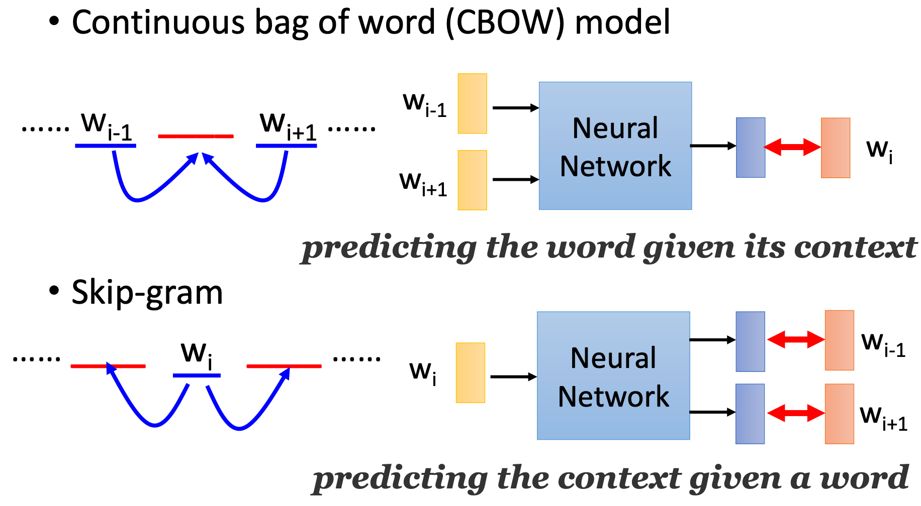
Negative Sampling

• Start with V random d-dimensional vectors as initial embeddings
• Train a classifier based on embedding similarity
  • Take a corpus and take pairs of words that co-occur as positive examples
  • Grab k negative examples for each target word
  • Train the classifier to distinguish these by slowly adjusting all the embeddings to improve the classifier performance

$\mathcal{L}_{neg} = -\log [P(+ \mid w_t, c_{\text{pos}}) \prod_{k=1}^K \log P(- \mid w_t, c_{\text{neg}_k})] = -\log \sigma(\mathbf{u}_{c_{\text{pos}}}^\top \mathbf{v}_{w_t}) - \sum_{k=1}^K \log \sigma(-\mathbf{u}_{c_{\text{neg}_k}}^\top \mathbf{v}_{w_t})$

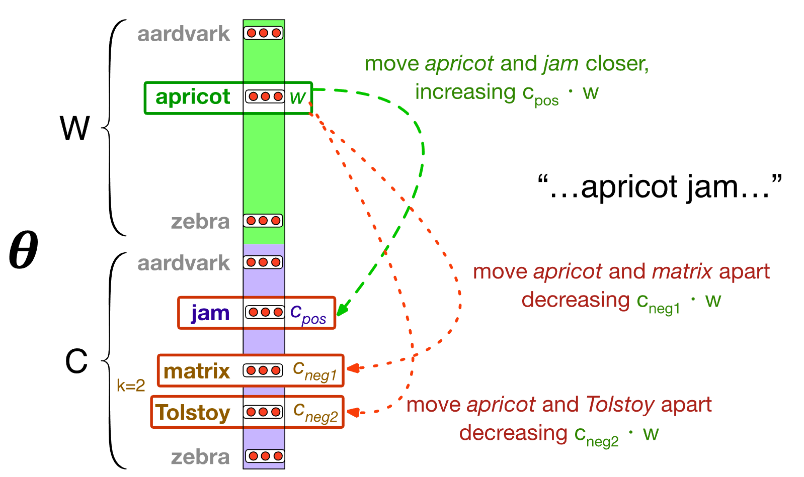
Where:

• $K$: Number of negative samples.
• $\mathbf{v}_{w_t}$: Input embedding of the target word $w_t$.
• $\mathbf{u}_{c_{\text{pos}}}$: Output embedding of the positive context word $c_{\text{pos}}$.
• $\mathbf{u}_{c_{\text{neg}}}$: Output embedding of a negative context word $c_{\text{neg}}$.

Hierarchical Softmax

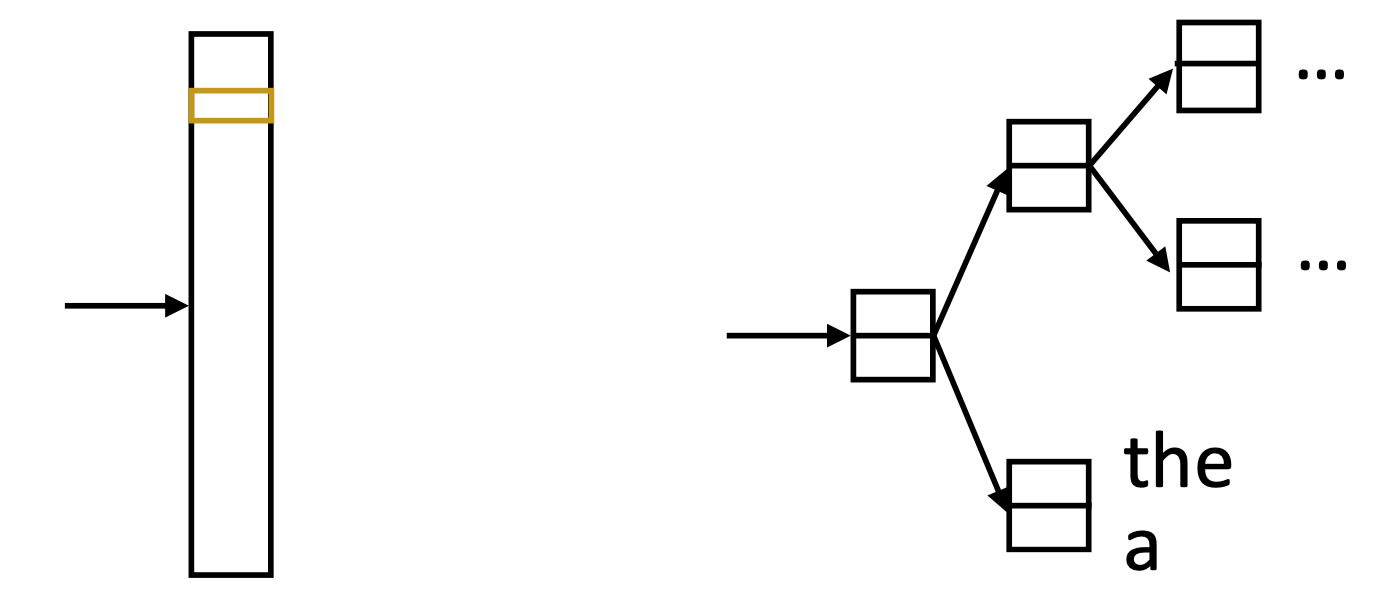
• Matmul + softmax over |V| (# of words) is very slow to compute for CBOW and SG
• Huffman encode vocabulary, use binary classifiers to decide which branch to take: log(|V|)

Golve

Construct a Global Vectors for Word Representation

Efficiency

• Pros: Efficient for large corpora
• Cons: Relatively slow for small or medium corpora

Effectiveness

• It is a kind of aggregated word2vec/CBOW
  • word2vec mainly focuses on local sliding windows
  • GloVe is able to combine global and local features
• More flexible with the values in matrix
  • log, PMI variants, ... many tricks can be played!

Sequence labeling

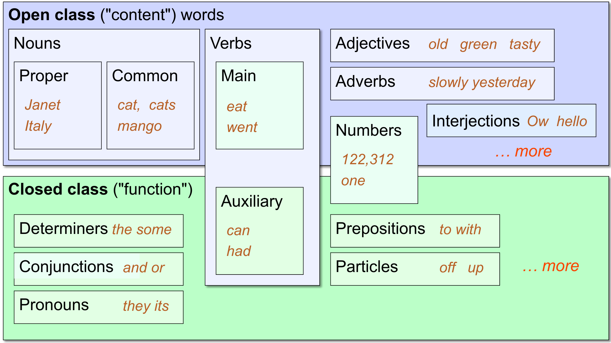
Part of Speech Tagging

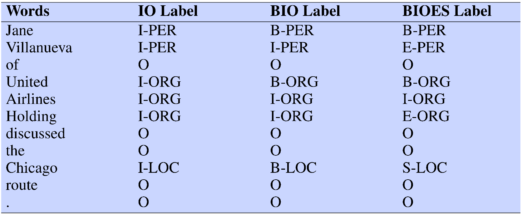
Named Entity Recognition

Most common

• PER (Person): “Marie Curie”
• LOC (Location): “New York City”
• ORG (Organization): “Stanford University”
• GPE (Geo-Political Entity): "Boulder, Colorado"

IO vs BIO vs BIOES

HMM(Hidden Markov Models)

Tag assignment: $\bold{w} = w_{1..n}, \bold{t} = t_{1..n}$

Bigram Assumption:

$$P(t_1, t_2, ..., t_n, w_1, w_2, ..., w_n) = P(t_1) \cdot \prod_{k} P(t_k \mid t_{k-1}) \cdot \prod_{k} P(w_k \mid t_k)$$

where

• Transition Probabilities $P(t_k \mid t_{k-1})$: The probability of transitioning from one state to another.
• Emission Probabilities $P(w_k \mid t_k)$: The probability of observing a specific observation given a state.
• $\bold{t}^* = \text{argmax}_t P(\bold{w},\bold{t})$