2 Deep Learning

Neural Network

Feed Forward Network

• Each perceptron in one layer is connected to every perceptron on the next layer
• Deep = Many hidden layers
• Last layer still logistic regression

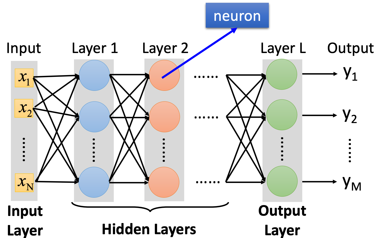
Perceptron(Neuron) $o = f(\sum_{k=1}^n i_kW_k)$, f is an activation function

• Identity: Linear Regression
• Sigmoid: Logistic Regression

One can stack perceptron to a Multi-layer perceptron(MLP)

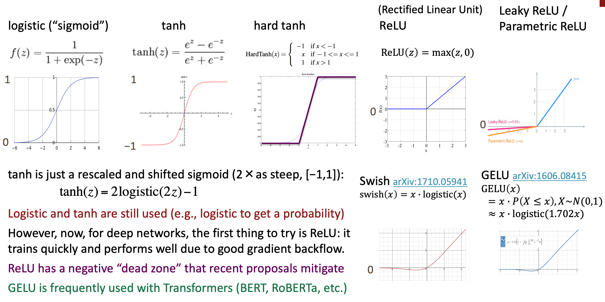
Activation functions

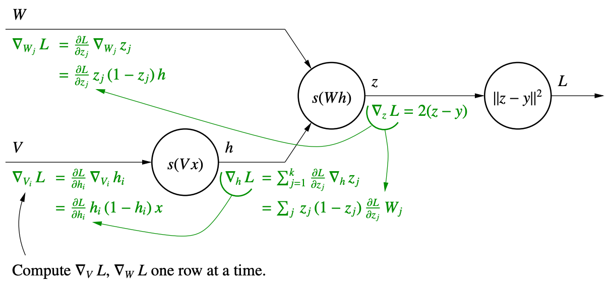
Feedforward and Backpropagation

• One forward pass: Compute all the intermediate output values
• One backward pass: Follow the chain rule to calculate the gradients at each layer, the calculate the product

Chain rule:

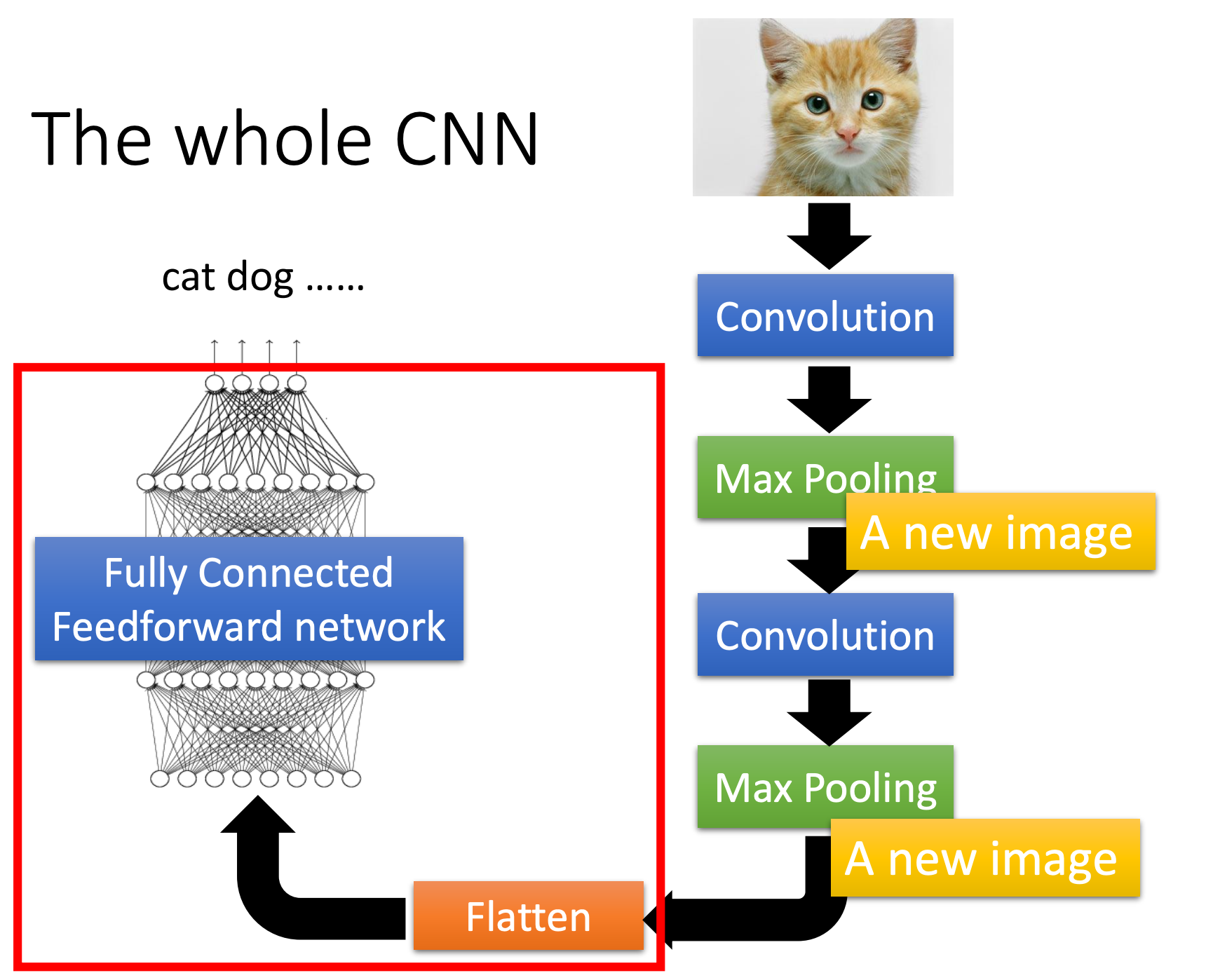
CNN

Why CNN for image:

• Some patterns are much smaller than the whole image
• The same patterns appear in different regions
• Subsampling the pixels will not change the object

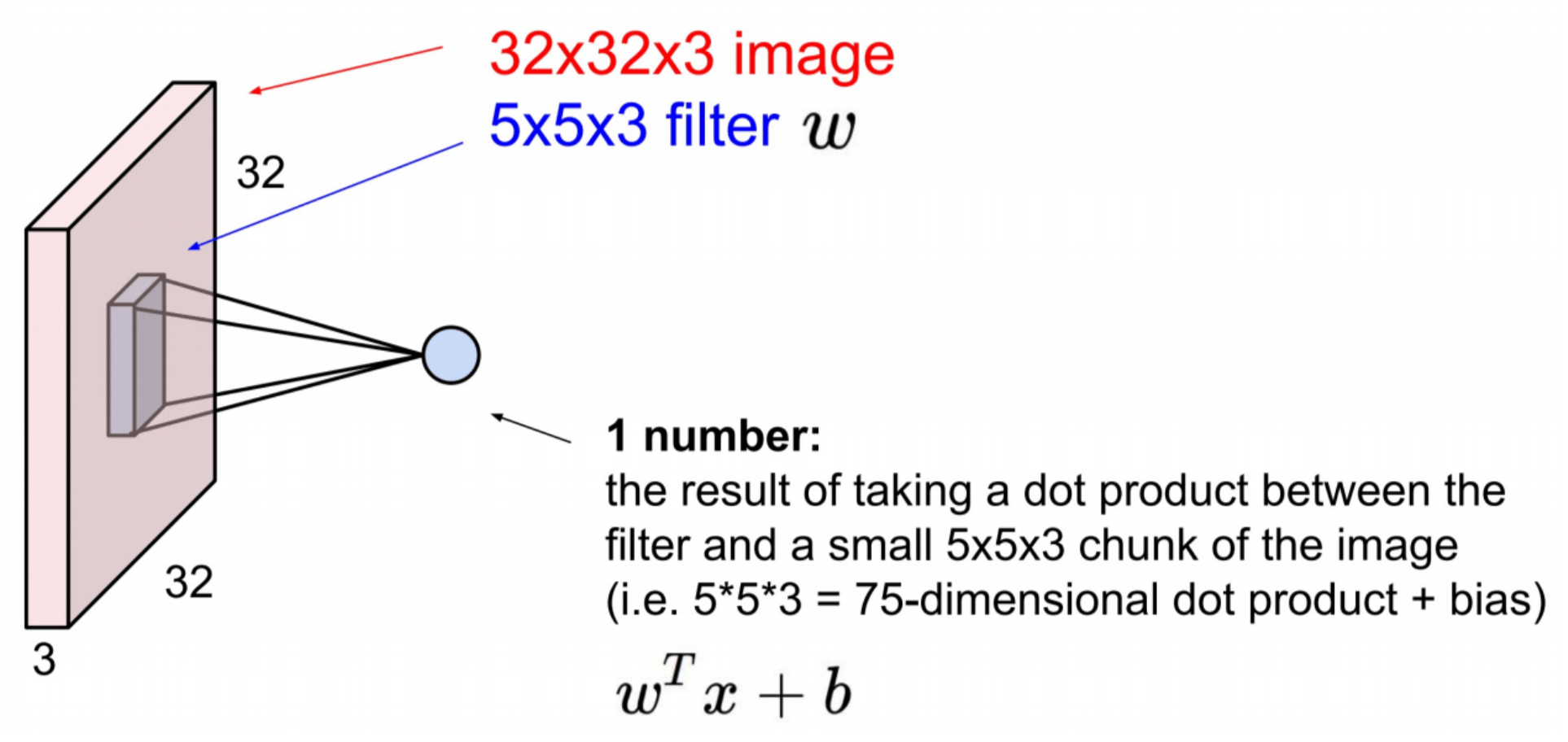
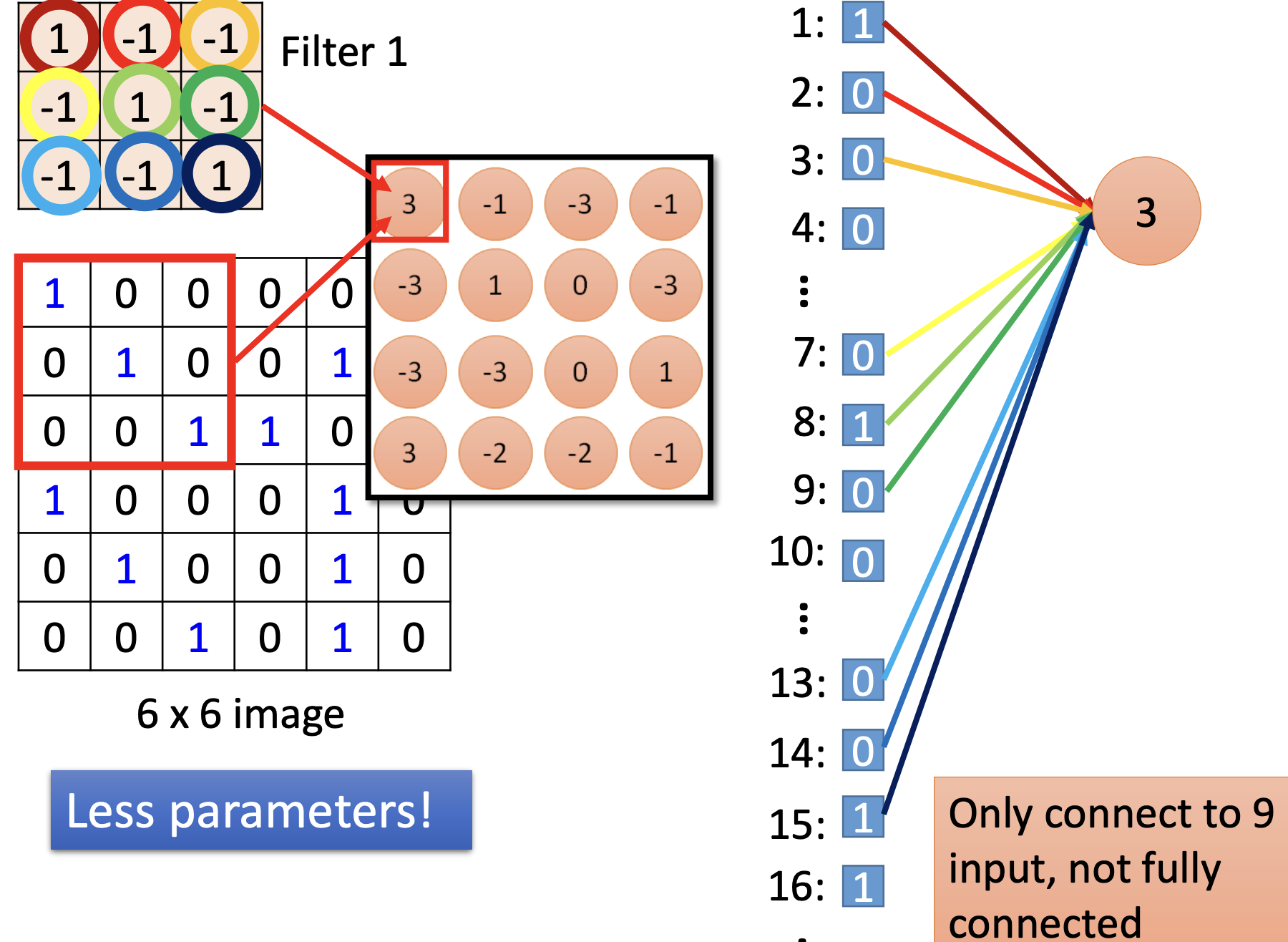
Convolution Layer

Convolutional Filters

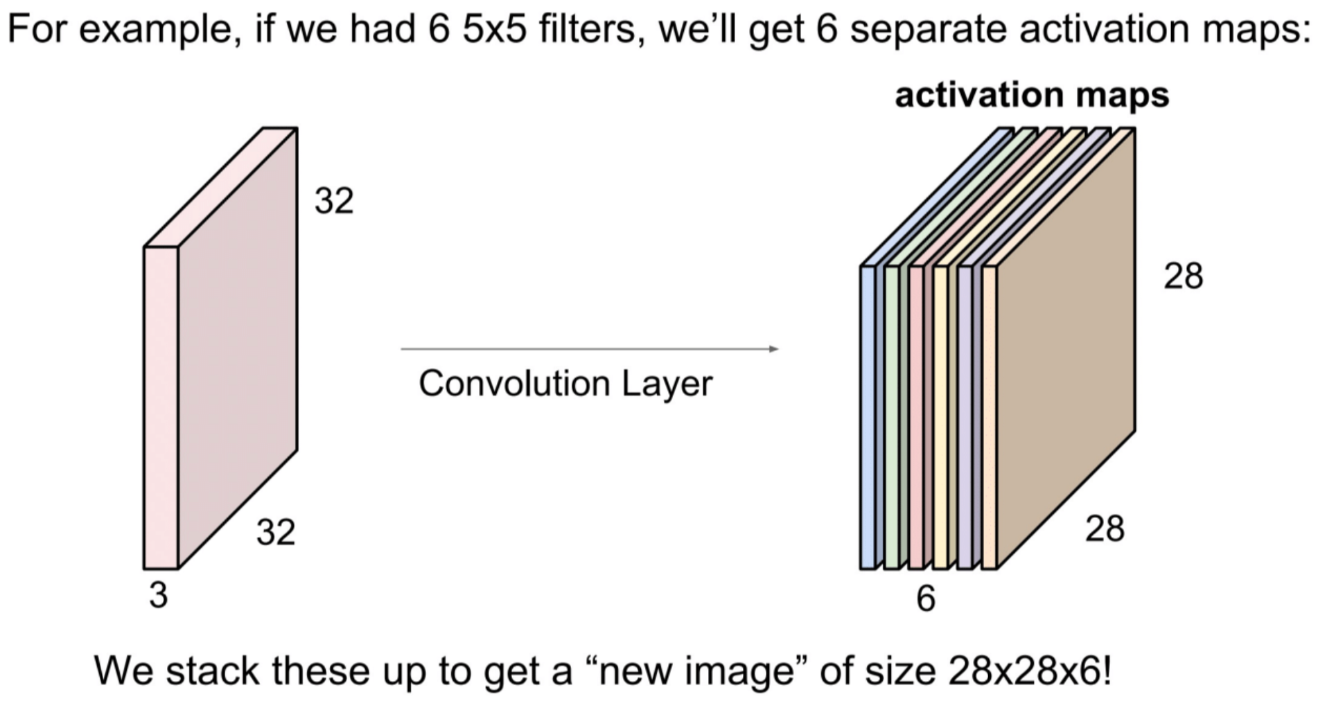
One can stack convolution filters into a new tensor, each filter is a channel

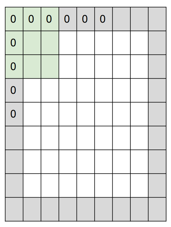
padding: Preserve input spatial dimensions in output activations by padding with n pixels border

Input: $W \times H \times D$ tensor

Hyperparameters:

• Number of filters: K, K is usually a power of 2 (32, 64, ...)
• Filter size: $F \times F \times D$, F is usually an odd number (e.g., 3, 5, 7)
• Stride: S, S describes how we move the filter
• Padding size: P

Output: $W' \times H' \times K$ tensor(Get the moving distance first, then add 1)

• W’ = (W – F + 2P) / S + 1
• H’ = (H – F + 2 P) / S + 1

Number of parameters: perform K times $w^Tx + b$: $(F\times F \times D + 1)\times K$

Usage: using 1*1 filters, we can keep the width and height but increase the number of channels.s

Pooling Layer

We can use Pooling as Subsampling(Downsampling)

Input: $W \times H \times D$ tensor

Hyperparameters:

• Filter size: $F \times F$
• Stride: S

Output: $W' \times H' \times D$ tensor

• W' = (W – F) / S + 1
• H’ = (H – F) / S + 1

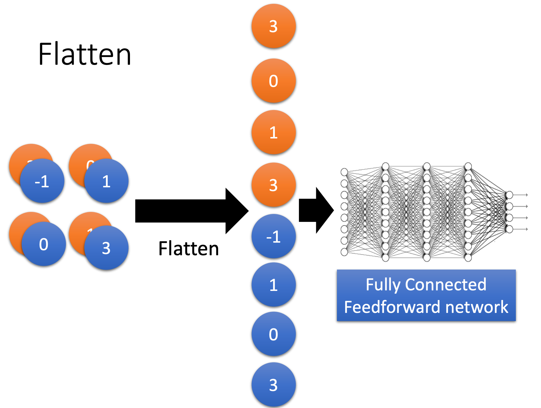
Fully Connected Layer

Flatten

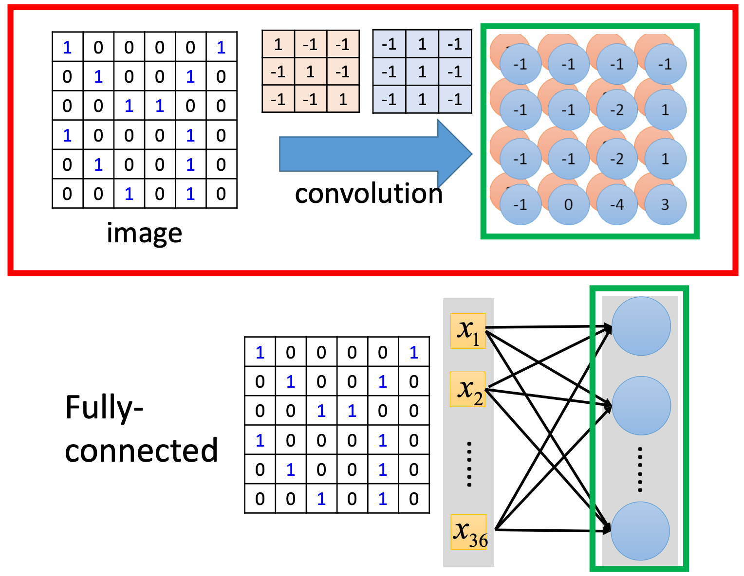
Convolution vs Fully connected

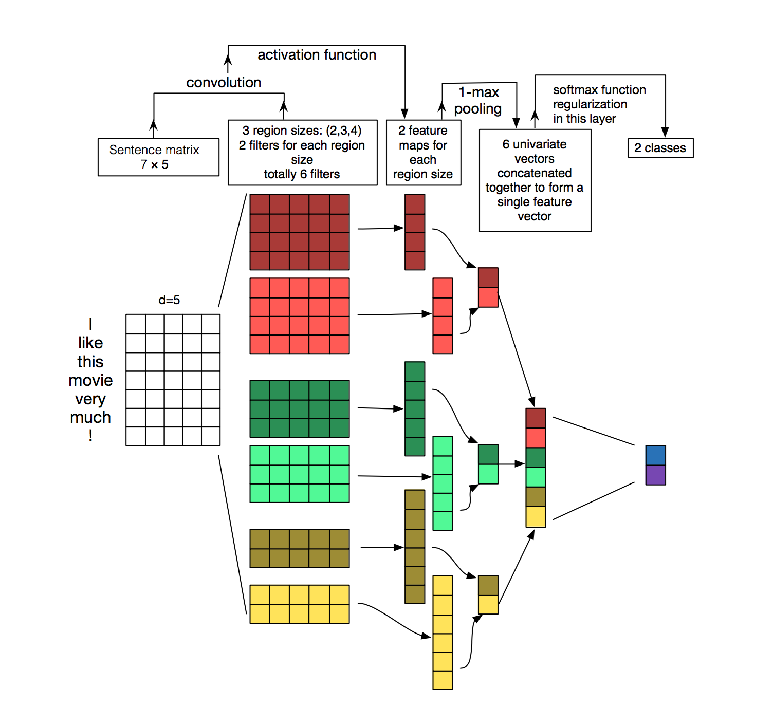
CNN for NLP

• kernel size: the other dimension not mentioned, e.g. $3(\times d)$
• parallel filters to get different views of the data that can be computed in parallel

RNN

Recurrent Neural Networks: Apply the same weights W repeatly

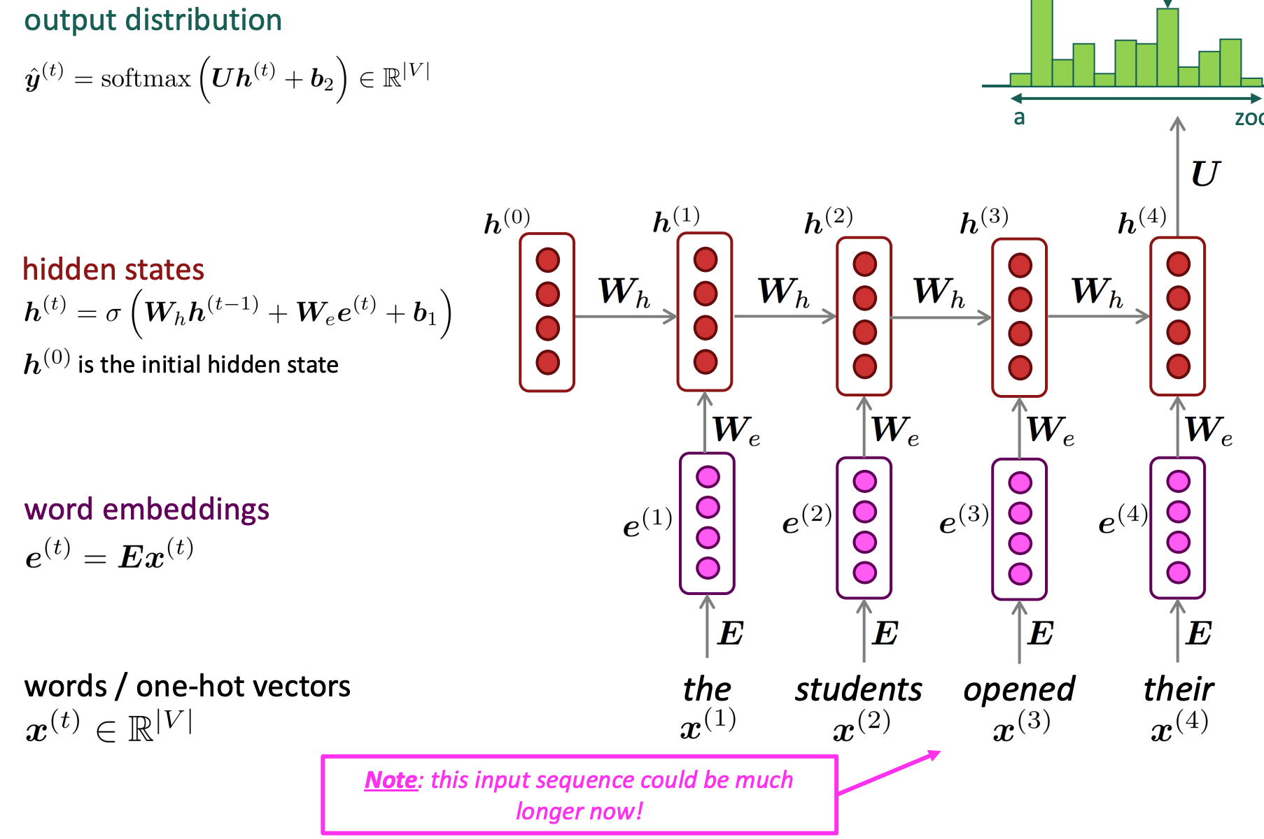
Advantages:

• Can process any length input
• Computation for step t can (in theory) use information from many steps back
• Model size doesn’t increase for longer input context
• Same weights applied on every timestep, so there is symmetry in how inputs are processed

Disadvantages:

• Recurrent computation is slow
• In practice, difficult to access information from many steps back

Vanishing and Exploding gradients

Vanishing gradients: model weights are updated only with respect to near effects, not long-term effects.

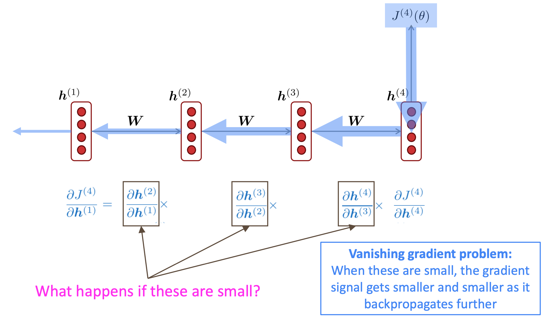
Exploding gradients: If the gradient becomes too big, then the SGD update step becomes too big. We take too large a step and reach a weird and bad parameter configuration.

Solution1: LSTM

Long Short-Term Memory RNN

On step t, there is a hidden state $h_t$ and a cell state $c_t$

• The cell stores long-term information
• The LSTM can read, erase(forget), and write information from the cell

$$\begin{aligned} f_t = \sigma{(W_fh_{t-1} + U_fx_t + b_f)} \\ i_t = \sigma{(W_ih_{t-1} + U_ix_t + b_i)} \\ o_t = \sigma{(W_oh_{t-1} + U_ox_t + b_o)} \\ c_t = f_tc_{t-1} + i_t\tanh(W_ch_{t-1} + U_cx_t + b_c) \\ h_t = o_t\tanh c_t \end{aligned}$$

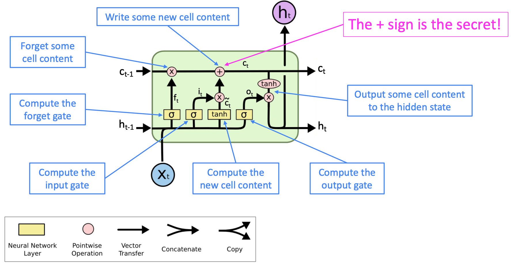
The LSTM architecture makes it much easier for an RNN to preserve information over many timesteps.

e.g., if the forget gate is set to 1 for a cell dimension and the input gate set to 0, then the information of that cell is preserved indefinitely.

Solution2: Other techniques

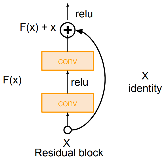
ResNet

The identity connection preserves information by default

Skip connection:

Say, halfway through a normal network, the activations are informative enough to classify the inputs well, but our chosen network still has more layers after that.

We can set weights to be zero(F(x) = 0), now the blocks could easily learn the identity function or small updates

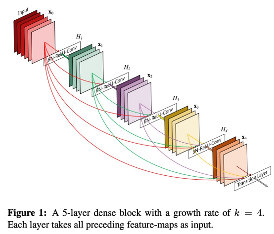
DenseNet

Directly connect each layer to all future layers

Bidirectional and Multi-layer RNNs

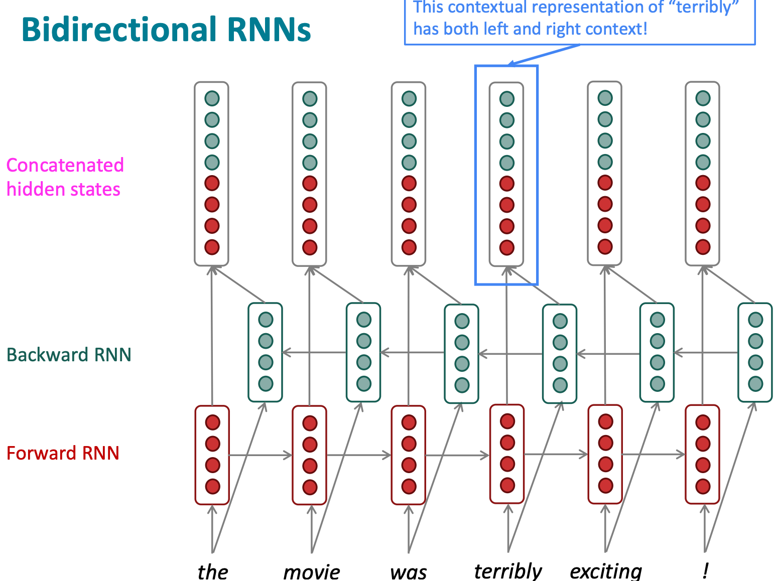
RNN could be a simple RNN or LSTM computation

Forward: $\overrightarrow{h_t} =$ RNN$_{FW}(h_{t-1},x_t)$

Backward: $\overleftarrow{h_t} =$ RNN$_{BW}(h_{t+1},x_t)$

Concatenated hidden states: $h_t = [\overrightarrow{h_t}; \overleftarrow{h_t}]$

Transformer

Problems with CNN/RNN

• Out of vocabulary
  • Solution: Tokenization with sub-words(e.g. ("h", "u", “man”))
• Non-contextual embeddings
• Non-attention
• Sequentiality
  • Solution: include sequential information(Positional embedding)

Architecture

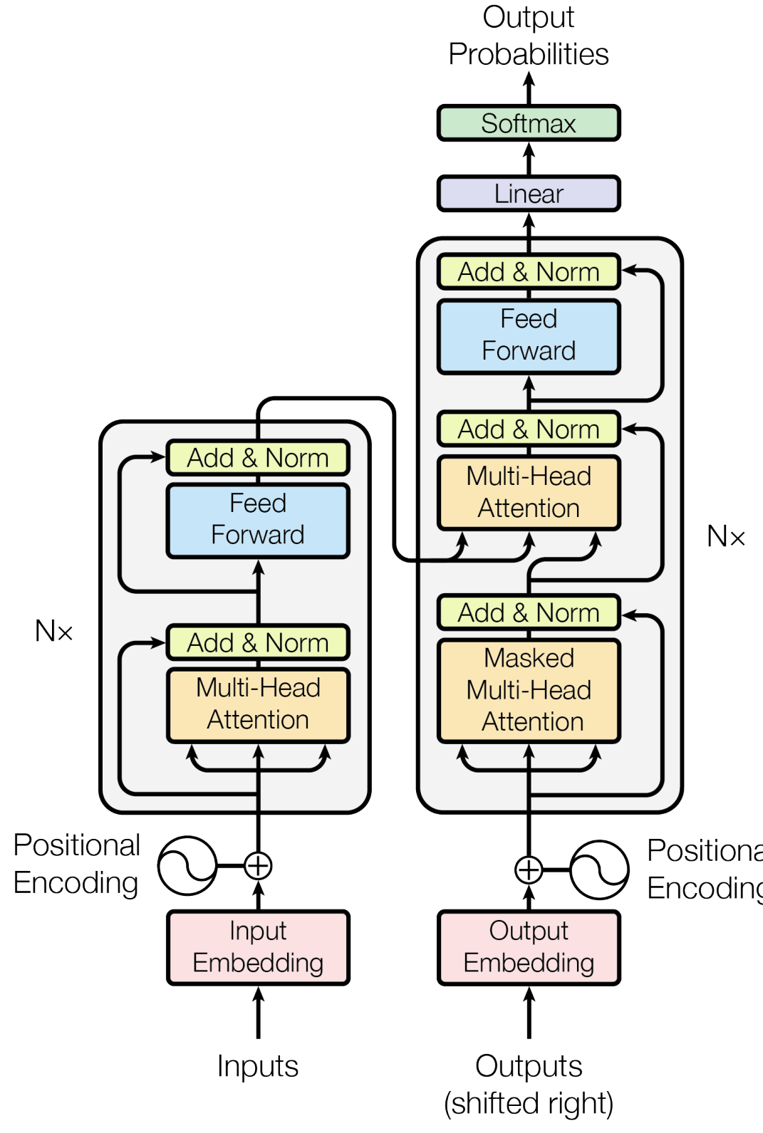
Attention

$$\text{MultiHead}(Q, K, V) = \text{Concat}(\text{head}_1, \dots, \text{head}_h) W^O$$

$$\text{head}_i = \text{softmax}(\text{mask}(\frac{QK^T}{\sqrt{d_k}}))V$$

$$Q = XW^Q, K = XW^K, V = XW^V, d_k = d_v = \frac{d_{\text{model}}}h$$

tip

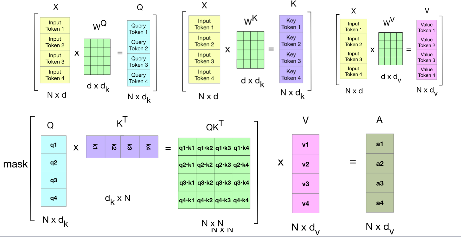
• Self-Attention: $Q = K = V$
• Cross-Attention: $Q$ comes from one sequence (e.g., decoder), and $K, V$ come from another sequence (e.g., encoder).

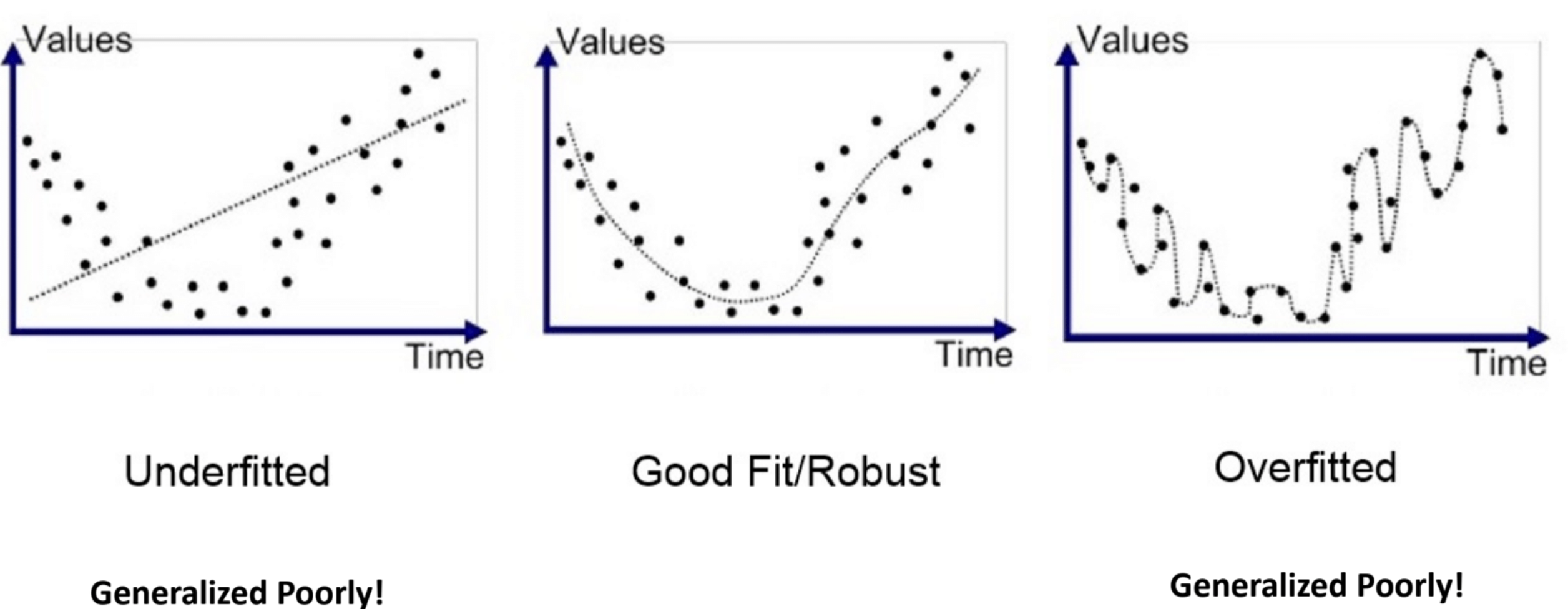
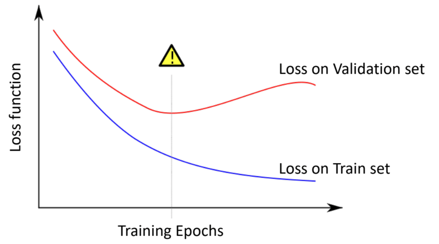
Overfitting

Early Stop

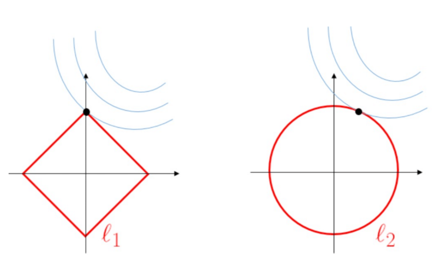
Weight regularization

L1 norm

Objective = $\alpha |\theta|$, we call it Lasso Regression

Gradient descent: More zeros in weights

L2 norm

Objective = $\beta |\theta|^2$, we call it Ridge Regression

Decay in weights: $\theta_{t+1} = \theta_{t} - \eta \nabla_{\theta} L(\theta_t)= (1-\lambda)\theta - \eta \nabla_{\theta} L(\theta_t)$

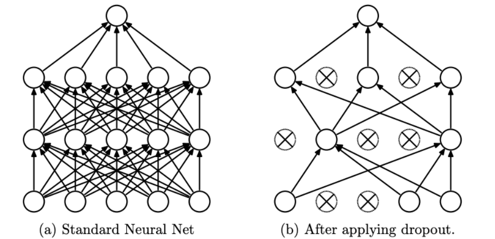
Dropout layer

Say dropout rate p.

During training, delete some intermediate output value with probability p or the weights times 1-p