2 Data Science

Numpy

• Slice
  • np.arrange(start,stop,step)
  • np.linspace(start,stop,num)
• Random
  • uniform: np.random.randint(low,high,size)
  • standard normal: np.random.randn(d1,d2,...)
• max,min
  • argmax, argmin return the indices of the maximum/minimum values

Ndarray

numpy shape is determined by the iteration of square brackets

a = np.shape(1) # shape:()
a = np.array([1, 2, 3, 4]) # shape: (4,)
a = a[:,np.newaxis] # array([[0],[1],[2]]),shape: (4,1)
b = np.shape([[1, 3]]) # (1,2)
c = np.array([(1,2),(3,4),(5,5),(423,12)],dtype=[('x', 'i4'), ('y', 'i4')])
print(c.shape, c.ndim) # (4,) 1
d = np.array([(1,2),(3,4),(5,5),(423,12)]) # shape: (4,2) ndim:2

indexing

## Elipsis
a = np.arange(120).reshape(2, 3, 4, 5)
print(a[:, :, :, 0])
print(a[..., 0]) # same
# [[[  0   5  10  15]
#   [ 20  25  30  35]
#   [ 40  45  50  55]]
# 
#  [[ 60  65  70  75]
#   [ 80  85  90  95]
#   [100 105 110 115]]]
print(a[0, :, :, 0])
print(a[0, ..., 0]) # same

Basic operation

elementwise vs dot

a = np.array([20, 30, 40, 50])
b = np.arange(4)
c = a + b # Matrix
print(c) # [20 31 42 53]
print(a*b) # same as np.multiply(): [0 30 80 150]
print(a.dot(b)) # same as np.matmul(): 260

With the larger dataset, we see that using NumPy results in code that executes over 50 times faster! Throughout this course (and in the real world), you will find that writing efficient code will be important; arrays and vectorized operations are the most common way of making Python programs run quickly.

Advanced Indexing

Index by arrays of indices

a = np.arange(12)**2  # the first 12 square numbers
i = np.array([1, 1, 3, 8, 5])  # an array of indices
print(a[i])  # array([ 1,  1,  9, 64, 25])
j = np.array([[3, 4], [9, 7]])  # a bidimensional array of indices
print(a[j])  # array([[ 9, 16],[81, 49]])

Index by boolean arrays

a = np.arange(12).reshape(3, 4)
a[a>4] = 0 # 0 is a matrix
print(a) # array([[0, 1, 2, 3],[4, 0, 0, 0],[0, 0, 0, 0]])

Deep copy

If a = b, that's only a reference

a = np.arange(int(1e8))
b = a[:100].copy()
del a  # the memory of ``a`` can be released.

Pandas

• pd.Series(data,index): One-dimensional ndarray with axis labels. data could be array-like, Iterable, dict, or scalar value
• pd.DataFrame(data,index,column): Two-dimensional, size-mutable, potentially heterogeneous tabular data.

Selection

• Select by column
• Slice the row
• Select by label

df = pd.DataFrame(
    {
        "A": 1.0,
        "B": pd.Timestamp("20130102"),
        "C": pd.Series(1, index=list(range(4)), dtype="float32"),
        "D": np.array([3] * 4, dtype="int32"),
        "E": pd.Categorical(["test", "train", "test", "train"]),
        "F": "foo",
    }
)
## 1. Select by column
print(df['A'])
# 0    1.0
# 1    1.0
# 2    1.0
# 3    1.0
## 2. Slice the row
print(df[0:2])
#      A          B    C  D      E    F
# 0  1.0 2013-01-02  1.0  3   test  foo
# 1  1.0 2013-01-02  1.0  3  train  foo
## 3. Select by label
print(df.loc[[0,2],['A','B']])
# Name: A, dtype: float64
#      A          B
# 0  1.0 2013-01-02
# 2  1.0 2013-01-02

MultiIndex

tuples = list(
    zip(
        ["bar", "bar", "baz", "baz", "foo", "foo", "qux", "qux"],
        ["one", "two", "one", "two", "one", "two", "one", "two"],
    )
)
index = pd.MultiIndex.from_tuples(tuples, names=["first", "second"])
df = pd.DataFrame(np.random.randn(8, 2), index=index, columns=["A", "B"])
#                      A         B
# first second                    
# bar   one     1.036623  0.775701
#       two    -0.491414 -0.596697
# baz   one    -1.039759  0.274683
#       two    -0.138051 -1.128008
# foo   one    -0.525837 -1.043091
#       two     0.152277  1.281915
# qux   one     0.625832  1.662615
#       two    -0.933067 -0.257373
print(df.loc['bar'].loc['one','B']) # 0.775701188641088
print(df.groupby('second').describe()['A'])
#         count      mean       std       min       25%       50%       75%       max
# second                                                                             
# one       4.0  0.523990  0.743125 -0.007540  0.125254  0.241141  0.639877  1.621220
# two       4.0  0.264113  0.644908 -0.414561 -0.175321  0.222076  0.661510  1.026859

Boolean Indexing

Selecting values from a DataFrame where a boolean condition is met

df = pd.DataFrame(np.random.randn(6, 4), index=pd.date_range("20130101", periods=6), columns=list("ABCD"))
print(df[df["A"] > 0])
#                    A         B         C         D
# 2013-01-02  0.945462 -0.880120  0.030657 -1.906303
# 2013-01-06  0.290602 -0.155123  0.174085 -1.606480

Operations

SQL join

left = pd.DataFrame({"key": ["foo", "foo"], "lval": [1, 2]})
right = pd.DataFrame({"key": ["foo", "foo"], "rval": [4, 5]})
print(pd.merge(left,right,on = 'key'))
#    key  lval  rval
# 0  foo     1     4
# 1  foo     1     5
# 2  foo     2     4
# 3  foo     2     5

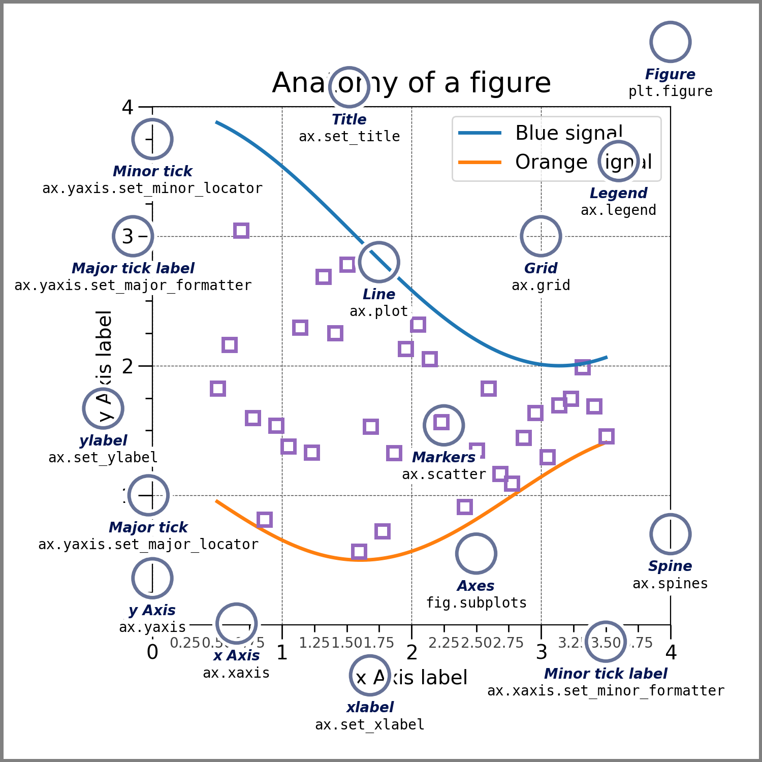
Matplotlib

The Figure keeps track of all the child Axes, an area where points can be specified in terms of x-y coordinates

fig, axes = plt.subplots()

plt.tight_layout()
fig, axes = plt.subplots(1,2,figsize=(8,2))
axes[0].plot(x,y1,'b:',x,y2,'g-')
axes[0].legend(['fig1','fig2'],loc='lower left')
axes[0].set_xlabel('x label')
plt.show()

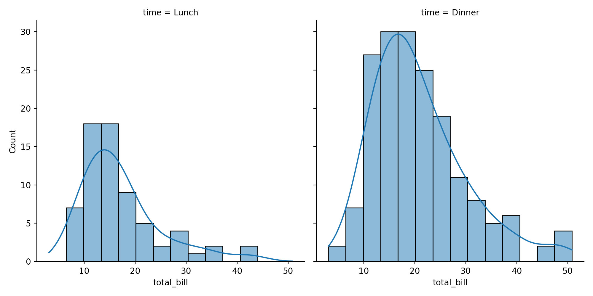
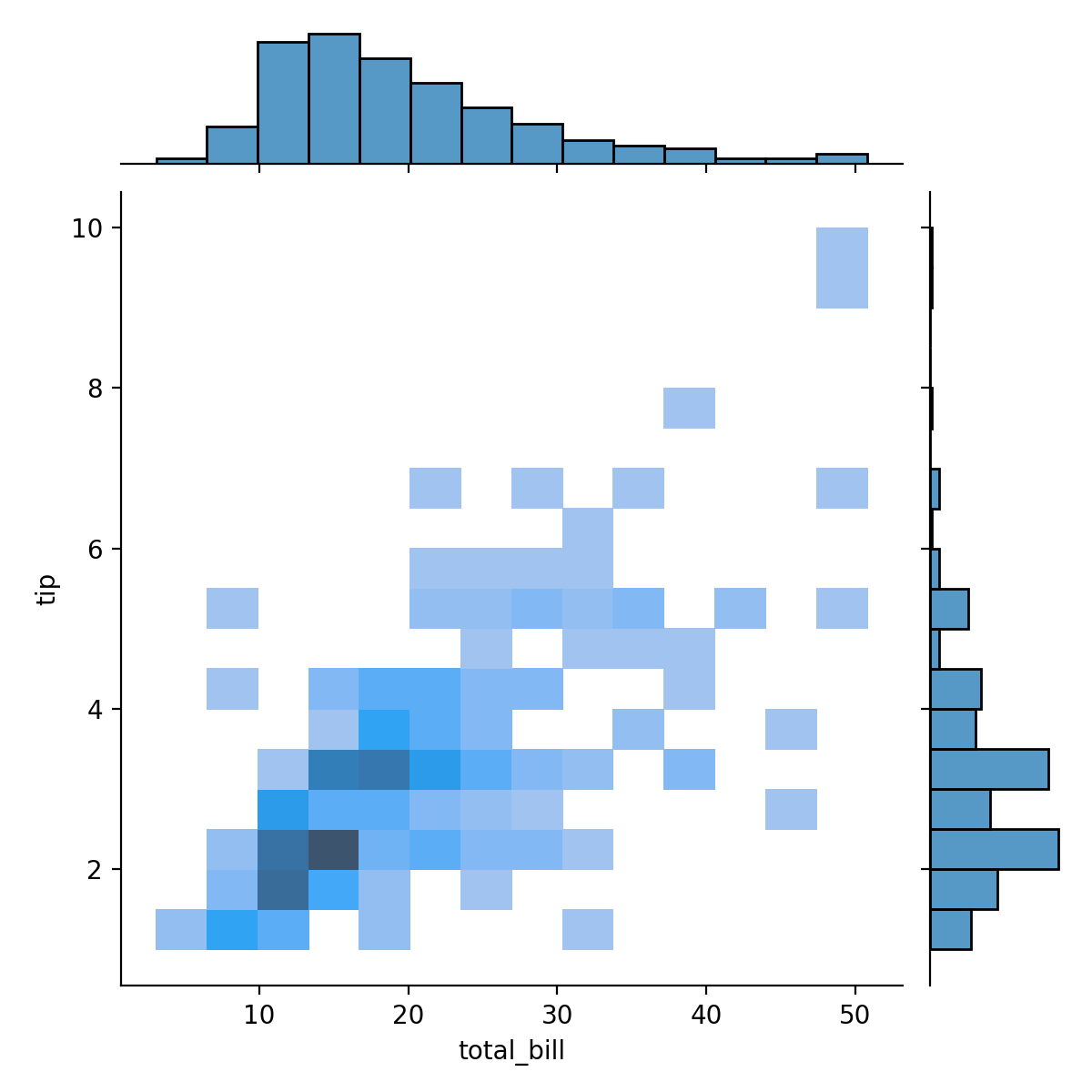
Seaborn

Distributional representations

KDE: kernel distribution estimation

tips = sns.load_dataset("tips")
sns.displot(data=tips, x="total_bill", col="time", kde=True)
sns.jointplot(x='total_bill',y='tip',data=tips,kind="hist")

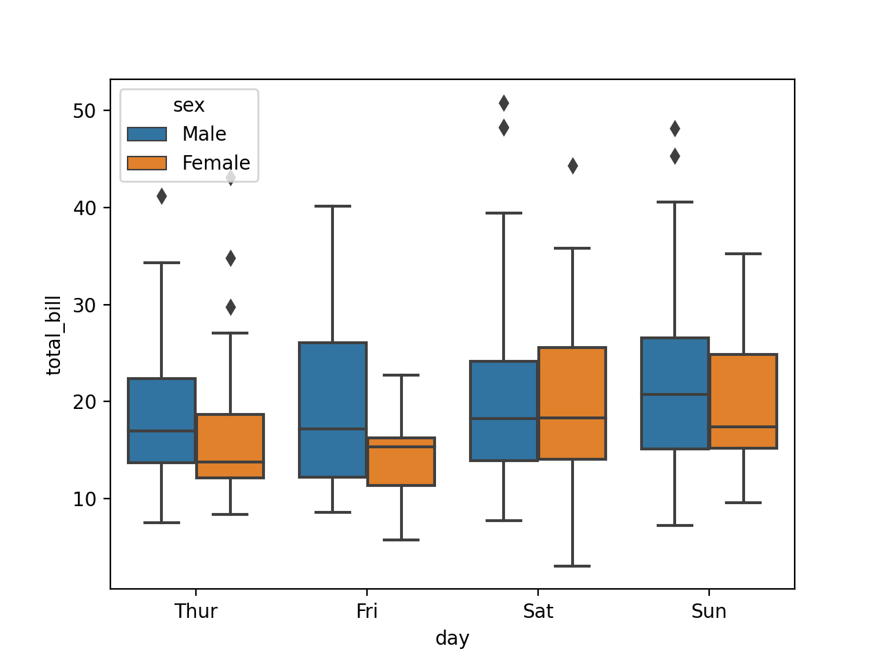
Catergorical Plot

tips =  sns.load_dataset("tips")
sns.boxplot(x='day',y='total_bill',data=tips,hue='sex')

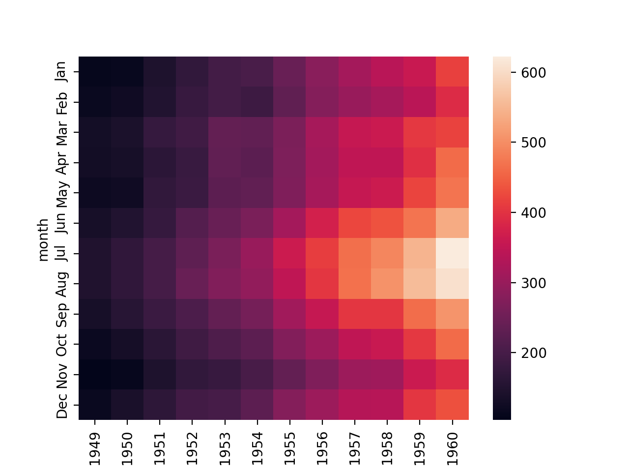
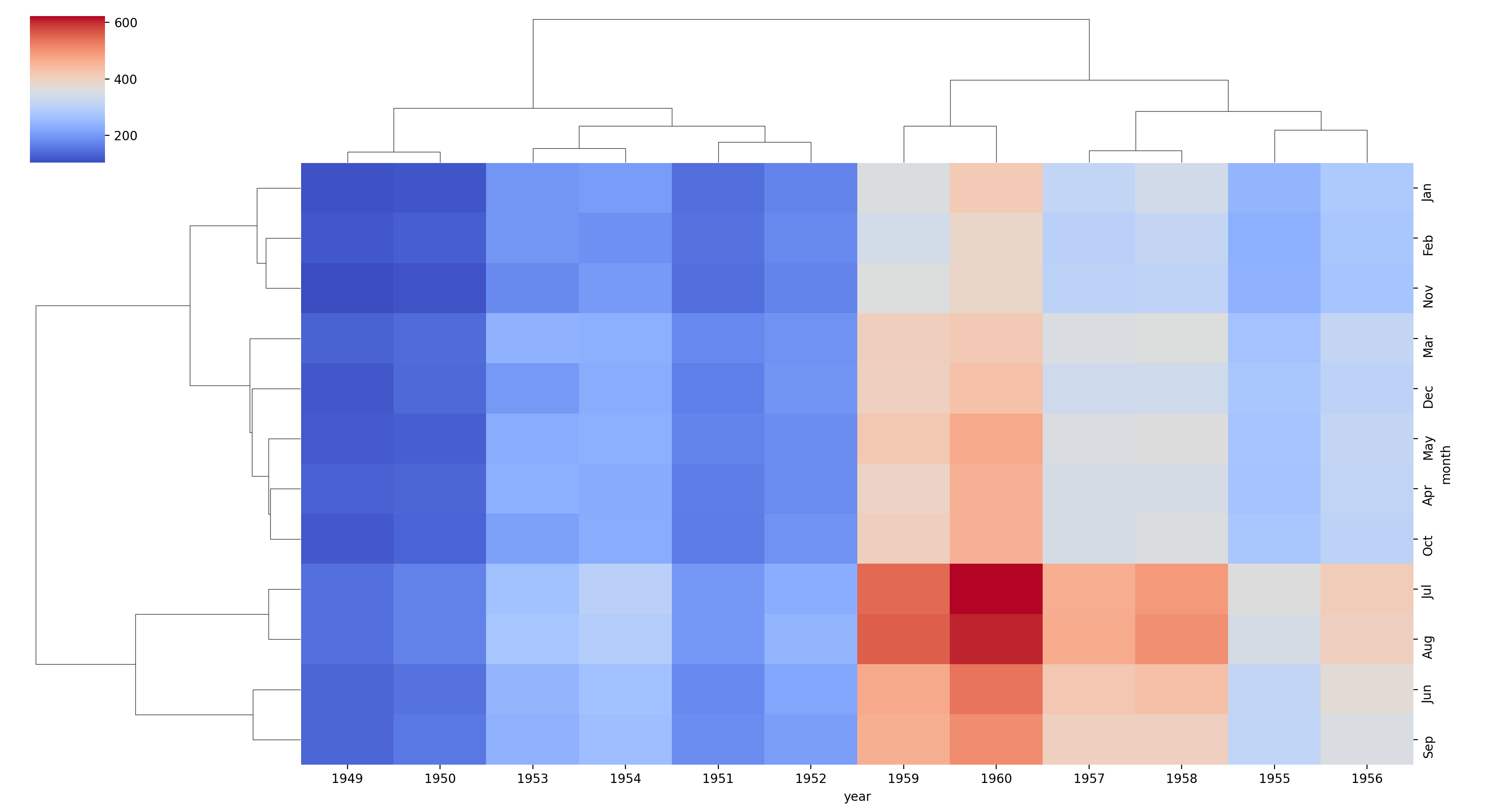
Matrix Plot

fp = flights.pivot_table(index='month',columns='year',values='passengers')
sns.heatmap(fp)
sns.clustermap(fp,cmap='coolwarm')